Statistics and AI Techniques for HCI
← Week 6Readings and resources
A mathematical reading for graduate Human Computer Interaction
An interface can make a task faster for some people, harder for others, and more pleasant without making it more accurate. A useful research conclusion therefore needs both a well-defined comparison and a statistical account of uncertainty. This reading develops that account from individual observations to estimates, tests, models, and sample-size planning. Its central question is how to make a defensible claim about an interface from a finite and imperfect set of observations.
The opening sections explain how experiments create interpretable data. Most of the reading concerns statistics: why variance uses squared deviations, why standard errors contain sample size, where t and F statistics come from, what confidence intervals and p-values mean, how power determines recruitment needs, and what bootstrap resampling actually estimates. Worked examples connect the mathematics to task time, success, errors, and reported experience. Regression and models for repeated observations extend the same ideas to richer HCI studies. A later chapter develops AI and machine learning as tools for analyzing experimental data, including participant-aware prediction, behavioral pattern discovery, signal analysis, and validated qualitative coding.
Only elementary algebra is assumed. Summation, probability, logarithms, and distribution notation are introduced when needed. Calculus is useful for understanding a probability density but is not required to reproduce the calculations. Numerical datasets explicitly labeled as teaching examples are fictional; they illustrate reasoning rather than report experimental findings.
By the end, you should be able to define the effect a study estimates, choose an analysis consistent with its design, reproduce basic calculations, explain uncertainty without overstating it, and recognize when a more specialized model is necessary. A small p-value cannot repair a confounded experiment, and a carefully designed experiment still needs an honest description of sampling uncertainty.
1 From a design question to an experiment
1 1 What would count as better
“Is this interface better?” is incomplete. Better for whom, on which task, after how much practice, using what equipment, and according to which outcome? Consider a university room-booking interface. Design A lists available rooms; Design B adds filters and a prominent confirmation summary. We might ask whether B reduces the time to make a correct booking, whether it reduces wrong-date bookings, or whether people feel more confident. Those are different questions, and they can have different answers.
An experiment deliberately varies a factor and observes outcomes under a defined assignment procedure. The interface is an independent variable or factor; A and B are its levels. Completion time is a dependent variable or outcome. Device, prior booking experience, task difficulty, and connection speed may affect the outcome even when they are not the factor of interest. A confound occurs when a competing explanation varies systematically with the condition, so that the intended effect cannot be separated from it.
A vacuum-cleaner comparison makes this concrete: a robotic cleaner could be faster yet leave more dirt. “Better cleaning” needs separate definitions of time, cleanliness, and possibly human effort. Giving the robot an easy room and the conventional cleaner a difficult room confounds the device with the environment. Giving an unfamiliar prototype to novices and a polished commercial product to experienced users mixes interface design, implementation maturity, and expertise. The comparison may still answer a useful first-use question, but it does not isolate the intrinsic superiority of an interaction technique.
Write an estimand before selecting a test. An estimand is the population quantity the analysis aims to estimate. In the booking example, let Δ be the population mean reduction in time, in seconds, when the relevant users complete comparable tasks with A and B under the specified protocol. We define a positive difference as an advantage for B:
This sign convention will be used in the paired-time example throughout the reading. For click rates, we will instead explicitly define the effect as the probability under B minus the probability under A. Always state the direction: an increase is beneficial for success but potentially harmful for errors or workload.
1 2 Discovery measurement and causal comparison
Formative evaluation seeks problems and explanations that help revise a design. Observing someone repeatedly search in the wrong menu can justify investigating the label even in a small study. Summative evaluation characterizes performance against a benchmark or compares alternatives. These are purposes, not rigid divisions between qualitative and quantitative data. A formative experiment can collect timing data; a summative study can include interviews. Systematic qualitative work is empirical evidence, not merely anecdote.
An observational association is also useful, but it answers a different question from random assignment. If experienced users choose keyboard shortcuts and finish faster, experience may explain both their choice and speed. Assigning comparable users to interaction techniques helps separate the technique from self-selection. Random assignment supports causal inference within the experiment; random sampling supports population representation. Neither automatically provides the other.
A controlled study can have strong internal validity while covering only a narrow population. A field study may capture realistic interruptions while leaving competing causes difficult to separate. Construct validity asks whether the measurement represents the intended concept. Reliability asks whether measurement is sufficiently consistent. External validity concerns transfer to other users, tasks, settings, and times. Statistical conclusion validity concerns whether the analysis and precision support the numerical claim. These questions should be considered together.
1 3 Independent and paired designs
In a between-participant design, different people use A and B. Random allocation distributes measured and unmeasured participant differences in expectation, not perfectly in every realized sample. Stratified randomization can balance a few important baseline characteristics, such as experience, while preserving random assignment within strata. Unequal allocation, such as 60:40, can also be randomized if it is planned and implemented correctly.
In a within-participant design, each person uses both interfaces. Each participant supplies a paired difference, reducing the influence of stable individual speed. The cost is possible learning, fatigue, transfer, and awareness of the comparison. Counterbalance A then B and B then A, and use comparable tasks whose answers cannot simply be remembered. Counterbalance task sets as well as interface order. A three-condition cyclic Latin square balances position but does not generally balance every first-order carryover. If exposure to one interface changes subsequent behavior irreversibly, a between-participant design may be preferable.
Repeated trials are not automatically independent participants. Twelve people performing ten tasks each produce 120 trial records, not 120 independent people. One analysis might average comparable trials within each participant and condition, giving twelve paired differences. Another might retain trials in a multilevel model. The choice changes the estimand and how task variation is represented; it must be explained rather than hidden inside a spreadsheet.
1 4 Recruitment and a usable protocol
Recruit people whose experience and access conditions are relevant to the claim. A student convenience sample can support conclusions about similar students under similar conditions; it does not establish usability for every population. Technical expertise is an exclusion criterion only when it conflicts with the target population. Professional developers are exactly the relevant users for some HCI systems. Recruitment procedures should accommodate assistive technologies, language needs, and participants who cannot use the default remote-study setup.
A systematic study-planning sequence provides a practical foundation: specify participants, tasks, success criteria, moderator behavior, recording, and analysis before the session; pilot the procedure; obtain informed consent; and debrief afterward. A goal such as “Book a room for four people tomorrow between 14:00 and 15:00” is more informative than instructions that reveal the intended sequence of clicks. State when timing starts and stops, how help is handled, and what constitutes a correct booking.
Think-aloud can reveal confusion, but speaking and prompting can alter performance. Timing under think-aloud remains measurable; its interpretation is timing under that protocol, not necessarily ordinary silent use. For a performance experiment, silent tasks followed by retrospective questions may be a better match. Use the same planned procedure across conditions, explain participation and recording clearly, minimize identifying data, and separate research participation from course grading or employment pressure. Ethical review and institutional requirements should be settled before recruitment.
2 Measurements and the data table
2 1 Match the outcome to the question
Completion time is continuous and nonnegative. Success is often binary. Error count is a nonnegative integer. Interface category is nominal. An ordered response such as very difficult through very easy is ordinal. A number stored in a cell does not by itself establish equal distances between response categories. These distinctions affect meaningful summaries and plausible statistical models.
For task success, specify the denominator: assigned participants, attempted tasks, completed sessions, or exposed users are not interchangeable. For error counts, define an opportunity or exposure when it varies: five errors in fifty actions differ from five in five hundred. For time, distinguish successful completion from abandonment, timeout, and instrument failure. Dropping failures can make a difficult interface look fast because only its successful users remain. A time-to-event analysis may be appropriate when incomplete tasks are censored; a completion-time analysis conditional on success must say so.
Questionnaires measure reported constructs. SUS summarizes perceived usability through ten items; with responses from 1 to 5, subtract 1 from each odd-numbered item, subtract each even-numbered item from 5, sum the ten contributions, and multiply by 2.5. The resulting 0–100 score is not a percentage of usability. Comparisons between systems are possible when population, tasks, administration, and interpretation are defensible. A published benchmark is context, not a universal pass threshold. [R10]
NASA-TLX measures perceived workload through mental, physical, and temporal demand, performance, effort, and frustration. Report whether you use the original weighting procedure or a raw unweighted version. Changing item wording or omitting dimensions changes the instrument. A preference score, success rate, and workload score can disagree without any measurement necessarily being wrong: they represent different aspects of interaction. [R11]
2 2 Preserve the unit of observation
A useful long-format trial table contains participant ID, randomized assignment or order, task ID, trial number, interface, start and end timestamps, success, error count, help, and missing-data reason. Keep the original records immutable and create derived analysis columns reproducibly. Use pseudonymous IDs rather than names in analysis files. Document units, coding, exclusions, and the direction of every scale.
The following fictional dataset is deliberately small enough to inspect by hand. Twelve participants each complete one matched booking task per interface after a fixed practice procedure. In this teaching example all tasks succeed. A/B order and task-set assignment are counterbalanced in the protocol; the numerical table is an illustration, not evidence that such balancing has actually been implemented in a real study.
| Participant | A time in seconds | B time in seconds | Difference A minus B |
|---|---|---|---|
| 1 | 52 | 44 | 8 |
| 2 | 65 | 59 | 6 |
| 3 | 47 | 49 | −2 |
| 4 | 80 | 65 | 15 |
| 5 | 59 | 55 | 4 |
| 6 | 72 | 60 | 12 |
| 7 | 54 | 54 | 0 |
| 8 | 90 | 72 | 18 |
| 9 | 61 | 54 | 7 |
| 10 | 68 | 65 | 3 |
| 11 | 75 | 65 | 10 |
| 12 | 57 | 58 | −1 |
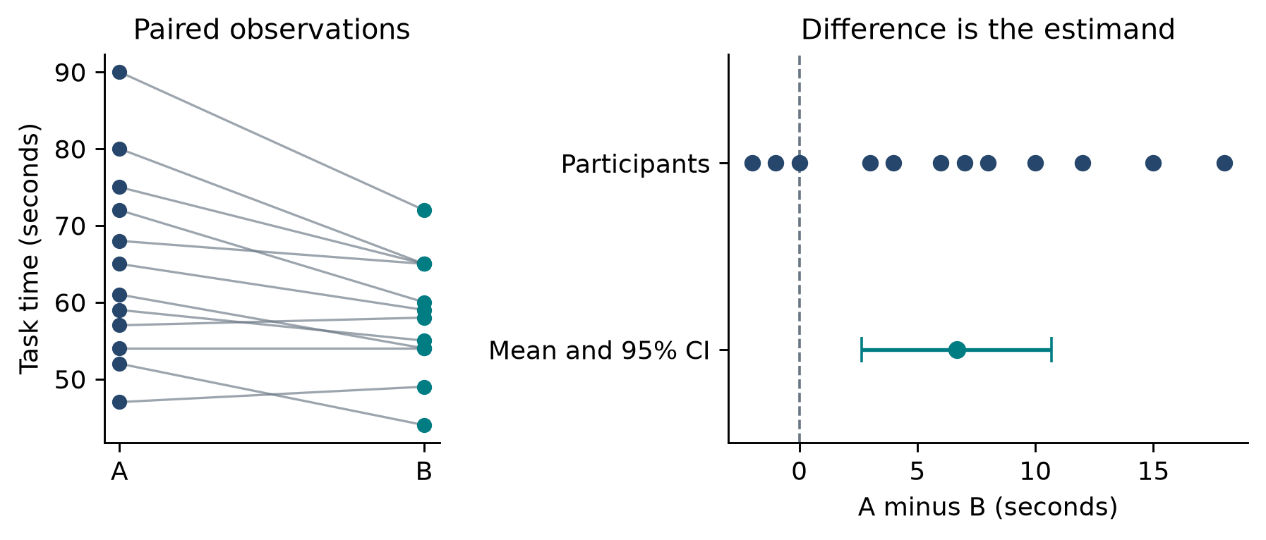
The A mean is 65.00 seconds and the B mean is 58.33 seconds. Their difference is 6.67 seconds, but the raw pattern matters: B is slower for participants 3 and 12 and unchanged for participant 7. A plot of only two bars would hide those observations and the pairing. The next sections build uncertainty estimates from the twelve differences rather than treating the two columns as unrelated samples.
3 Descriptive statistics and the origin of standard error
3 1 Mean median and spread
For observations x₁ through xₙ, the arithmetic mean and sample variance are
The mean uses every numerical value and estimates the expected value under a sampling model. The median is the middle ordered value, or the average of the two middle values for an even sample size. It describes the 50th percentile and is less sensitive to extreme observations. Neither is universally superior: expected resource use may require a mean, while typical task performance may be communicated well by a median. Report the question the summary answers.
For times 10, 12, and 14 seconds, the mean is 12. Deviations are −2, 0, and 2; their sum is zero. Squaring prevents cancellation and produces a sum of squares of 8. Sample variance is 8/2 = 4 seconds², and sample standard deviation is 2 seconds. Variance is useful algebraically because variances of independent sums add; standard deviation restores the original measurement unit for interpretation.
If these three observations were the entire finite population of interest, its descriptive variance would be 8/3 seconds². When estimating the variance of an underlying distribution from independent observations, the divisor n−1 corrects for estimating the center from the same sample. This is not an arbitrary safety margin and is not based simply on the claim that small samples miss extreme values.
3 2 Why the divisor is n minus one
The deviations from the sample mean obey a constraint: their sum is zero. Once n−1 deviations are known, the last is determined. This is the first encounter with degrees of freedom, the number of independent pieces of variation left after fitted quantities impose constraints.
The following identity gives a more precise explanation. Let μ and σ² denote the population mean and variance. For independent identically distributed observations with finite variance,
Taking expectations, the first term on the right contributes nσ². The second contributes n Var(x̄) = σ² because Var(x̄) = σ²/n. The expected sample sum of squares is therefore (n−1)σ². Dividing by n−1 gives an unbiased estimator of σ². Taking its square root gives the conventional sample standard deviation, but the square root itself is not exactly unbiased for σ. Normality is not required for this variance identity; independence, a common distribution, and finite variance are doing the work.
3 3 Why the t test denominator contains n
Standard deviation describes variability among observations. Standard error describes variability of an estimator across repeated samples. Suppose X₁ through Xₙ are independent with common variance σ². The variance of their average is
Consequently the standard deviation of the sampling distribution of the mean is σ/√n. Since σ is usually unknown, we estimate it with s:
If individual task times have standard deviation about 12 seconds, a sample of 9 independent users has estimated mean SE about 4 seconds, whereas a sample of 36 has SE about 2 seconds. Quadrupling n approximately halves uncertainty in the mean; it does not make individual people twice as consistent. Larger samples reduce random sampling error while leaving systematic bias untouched.
The extra n is essential. Replacing s²/n by s² changes uncertainty about an average into dispersion among individuals. If SS denotes the sum of squared deviations, the same term can be written SS/[n(n−1)], because s² = SS/(n−1). Substituting a sum of squares does not remove the sample-size adjustment.
3 4 Dependence changes the mathematics
For correlated observations, variance includes covariance terms:
Measurements from one person are often positively correlated. Ignoring that dependence usually understates uncertainty. Under a simple equal-cluster model with m observations per cluster and intraclass correlation ρ, the design effect is approximately 1+(m−1)ρ. With 10 trials per person and ρ=.5, it is 5.5. This approximation illustrates why counting trials as independent users can badly exaggerate precision; actual repeated-measures analyses should model their design rather than mechanically substitute an effective sample size.
For a paired difference D=A−B, covariance can help:
People who are generally slow on A may also be slow on B. Subtracting within each person removes some of that stable variation. This statistical advantage explains the attraction of paired designs, but it does not remove learning or carryover bias.
4 Probability and sampling distributions
4 1 Outcomes statistics and distributions
A random variable describes an uncertain numerical outcome. Its probability distribution assigns probabilities to discrete values or probability density to continuous values. A density's height is not a probability: probability is area under the curve over a range. The total probability is one. A parameter such as μ or a success probability π characterizes a population model; a statistic such as x̄ or an observed success proportion estimates it from data.
For one binary outcome X, with success probability π, X follows a Bernoulli distribution. Its mean is π and its variance is π(1−π). For n independent trials with the same probability, the total success count K has a binomial distribution:
The observed proportion is π̂=K/n, so its variance is π(1−π)/n. A coin-toss count is exactly binomial under these assumptions, not exactly normal. A normal approximation becomes useful when the expected success and failure counts are sufficiently large for the particular calculation. Extreme probabilities, small samples, or dependent trials can make the approximation poor.
4 2 The distribution of observations is not the distribution of means
The raw time distribution describes individual participants. A sampling distribution describes a statistic across repeated studies of the same size under the same sampling mechanism. It is a conceptual distribution even when we only conduct one study. For normally distributed independent observations, the sample mean is normal for every n. More generally, a central limit theorem gives an approximate normal distribution for a standardized mean as n grows under appropriate conditions, including finite variance in the usual independent identical-distribution setting.
There is no universal n=30 guarantee. Severe skew, heavy tails, dependence, and rare events affect the adequacy of the approximation. Nor does computing more simulated means change the sample size inside each mean. Ten thousand bootstrap samples of size three give a detailed approximation to a small-sample bootstrap distribution, which can remain irregular or discrete.
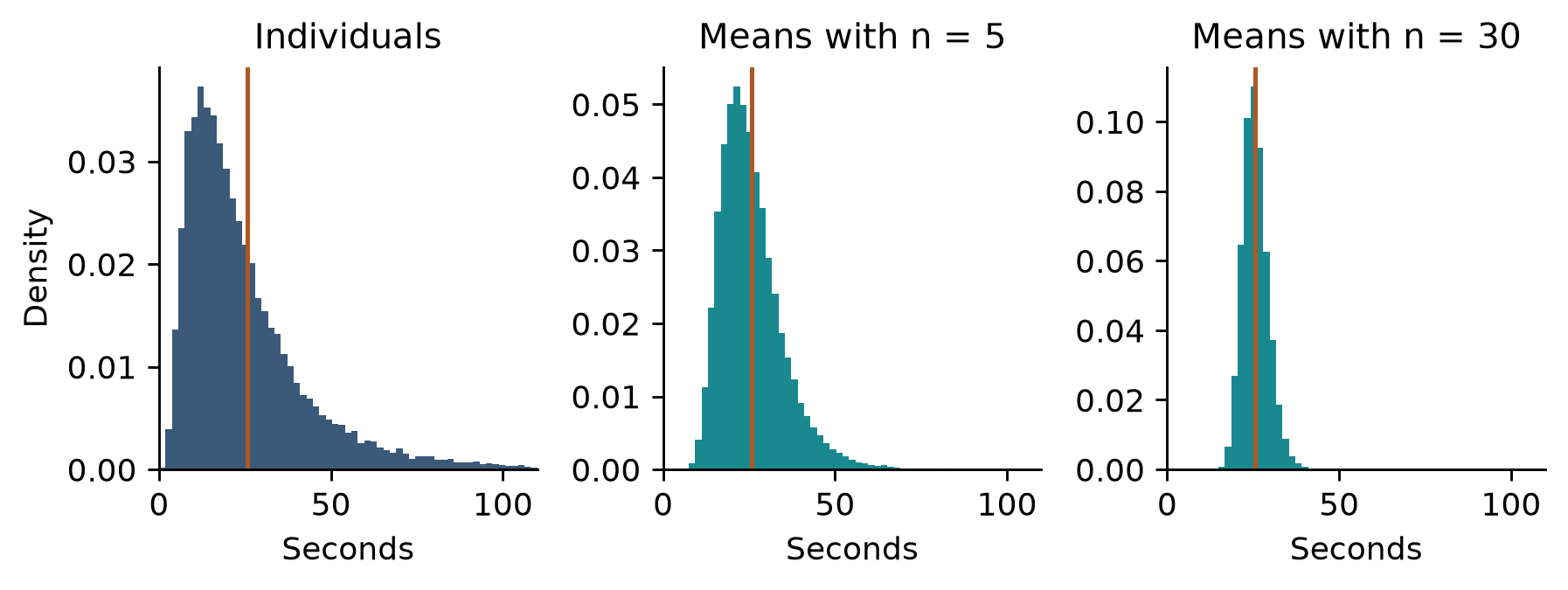
A bimodal population can have a mean between its peaks without the mean being mathematically invalid. Suppose equally common groups complete a task near 20 and 120 seconds. The mean near 70 seconds summarizes expected time, although it describes neither group's typical experience. Show the distribution and investigate relevant subgroups rather than declaring the average false or expecting bootstrap resampling to solve the interpretive problem.
4 3 Normal t chi square and F distributions
The standard normal distribution has mean zero and variance one. A standardized mean uses its standard error to express how far an estimate lies from a reference value. When σ is known and observations are normal, Z=(x̄−μ₀)/(σ/√n) follows the standard normal distribution under the null hypothesis μ=μ₀.
Estimating σ introduces additional uncertainty. For an independent normal sample, the standardized mean using s follows Student's t distribution with n−1 degrees of freedom:
Small-degree t distributions have heavier tails than the normal distribution, so an equally rare standardized observation must be farther from zero. As degrees of freedom increase, t approaches the standard normal. The familiar 1.96 multiplier is therefore not the correct 95% critical value for every small-sample mean.
A sum of ν independent squared standard normal variables has a chi-square distribution with ν degrees of freedom. For a normal sample, (n−1)S²/σ² has this distribution. The ratio of two independent chi-square quantities after dividing each by its degrees of freedom has an F distribution:
ANOVA uses this ratio to compare variation associated with group means to variation remaining within groups. F is nonnegative and has two degrees-of-freedom parameters. Its critical-value table specifies a tail probability under a null model. That table alone does not tell us the required sample size; power also needs a specified alternative effect and noise level.
5 Estimation confidence intervals and hypothesis tests
5 1 Estimate an effect before classifying a result
The point estimate is the best single numerical summary supplied by the chosen estimator. An interval adds uncertainty. Many familiar confidence intervals take the form estimate ± critical value × standard error, although not every valid interval has this symmetric form. For the mean of independent normal observations with unknown variance,
A 95% confidence procedure covers the fixed population parameter in 95% of repeated samples under its assumptions. Once a particular interval is calculated, its endpoints are fixed; the frequentist statement is about the procedure's long-run coverage. In ordinary reporting, “the estimated effect is 6.67 seconds, with a 95% confidence interval from 2.65 to 10.68 seconds” is clear. Avoid converting that interval into a 95% probability that a fixed parameter lies inside it. A Bayesian credible interval has a different interpretation and requires an explicit prior and likelihood. [R2]
A confidence interval for a mean is not a minimum–maximum range of individual performance. Under a simple independent normal model, a prediction interval for one future observation is wider:
The extra 1 represents the variability of the new observation itself. A tolerance interval answers yet another question: it aims to cover a specified fraction of a population with a specified confidence level. Do not use a confidence interval for average time to promise that 95% of people finish inside its limits.
5 2 Alpha is a design choice and p is a calculated tail area
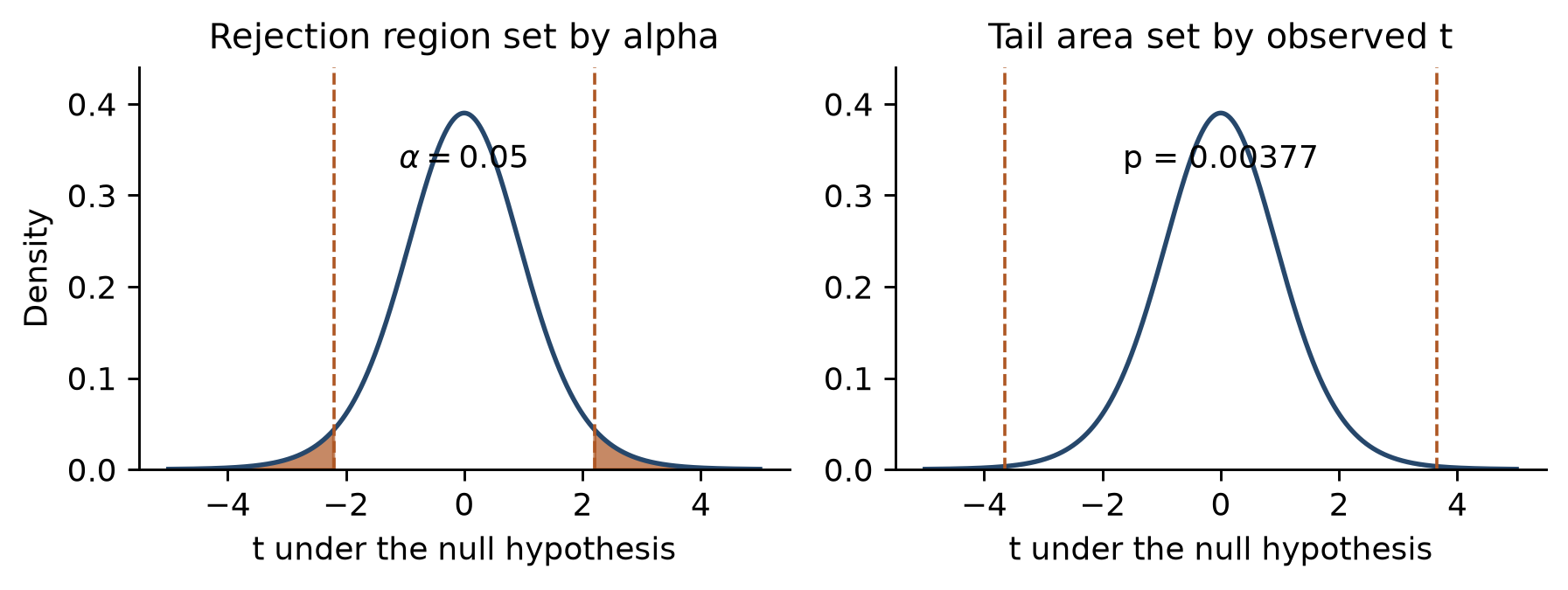
A null hypothesis specifies a parameter value or set of values, such as H₀:Δ=0. A two-sided alternative considers both positive and negative departures. Choose a statistic whose extreme values would be inconsistent with the null, then calculate how often the specified null model produces values at least as extreme as observed. For a symmetric t test,
Here F with a subscript denotes a cumulative distribution function, not an ANOVA F statistic. The p-value is conditional on the null and the rest of the statistical model. It is not P(H₀|data), not the probability the data were “caused by chance,” and not the probability that a deployment decision is wrong. The ASA statement emphasizes these interpretive limits and the need to consider effect magnitude and study context. [R1]
Alpha is the chosen Type I error rate of a testing procedure: the probability of rejecting a true null under its assumptions. It is fixed before examining the relevant results. With α=.05, the procedure falsely rejects in about 5% of repeated experiments in which the null is true; it does not mean that 5% of all significant findings are false. That latter fraction also depends on which hypotheses are investigated, power, selection, and reporting practices.
5 3 Direction error and absence of evidence
A one-sided alternative tests a prespecified direction. For H₁:Δ>0, p=1−F(tobs). If the estimate goes strongly in the opposite direction, the one-sided p-value should be large, not half a small two-sided value. Choosing a direction after seeing the sign invalidates the intended error control. One-sided testing also does not excuse ignoring harmful results; those still require reporting and interpretation.
Failing to reject H₀ does not establish that interfaces are identical. A wide interval may include no effect and substantial effects in either direction. A narrow interval near zero may instead rule out effects of practical interest. The interval explains the difference between uninformative evidence and evidence of a small effect. For a matching two-sided test and confidence interval, rejecting at α=.05 corresponds to a 95% interval excluding the null value. This equivalence should not be assumed between unrelated tests and intervals.
Statistical and practical importance are separate. A very large experiment can precisely estimate a 0.1-second change; a small study can estimate a much larger change imprecisely. Define a smallest effect of interest from task cost, user burden, or research theory. A change may be worthwhile for a frequently repeated action and negligible for a rare action. Neither p=.049 nor p=.051 changes the underlying usability argument abruptly.
6 Comparing means with t tests
6 1 The one sample t test
Suppose a benchmark defines mean time μ₀=60 seconds under a genuinely comparable protocol. An independent sample has mean 54, standard deviation 12, and n=16. The estimated standard error is 12/4=3 seconds; the statistic is (54−60)/3=−2 with 15 degrees of freedom. A two-sided test gives p≈.0639, and the 95% interval is 54±2.131×3, or [47.61,60.39] seconds. The estimate suggests a reduction, but this interval still includes the benchmark.
The benchmark is treated as fixed in this calculation. If “60 seconds” came from another finite sample, its uncertainty usually belongs in a two-sample analysis. Comparing a new group to last year's observed average also invites confounds from population, task, or system changes. A one-sample formula cannot make a historical comparison randomized.
6 2 A complete paired calculation
For the booking data, calculate dᵢ=Aᵢ−Bᵢ for each participant. The paired test is a one-sample t test on these differences:
Here n=12, Σdᵢ=80, and Σdᵢ²=972. A computational identity makes the arithmetic easy to check:
Therefore s²d=438.6667/11=39.8788 seconds², sd=6.315 seconds, and SE=6.315/√12=1.823 seconds. Testing Δ₀=0 gives t=6.6667/1.823=3.657 with 11 degrees of freedom. The two-sided p-value is .00377. Using t.975,11=2.201, the interval is
An appropriate interpretation is that B reduced mean task time in this fictional matched-task comparison, with the stated uncertainty under the paired model. It does not follow that every person benefits, that success rates improve, or that the effect generalizes to untested populations. If 5 seconds were the smallest practically worthwhile reduction, the interval crosses that threshold: the evidence for some improvement is stronger than the evidence for an improvement of at least 5 seconds.
The standardized paired effect dz=d̄/sd is about 1.056. This describes the mean change in units of the difference-score standard deviation. It is not numerically interchangeable with an independent-groups Cohen d. Report seconds alongside any standardized effect, name the standardization, and provide uncertainty for the effect rather than classifying it solely with generic “small” and “large” labels.
For exact small-sample inference, the differences should be independent across participants and normally distributed. The two raw columns do not each need to pass a separate normality test for this paired assumption. Inspect a difference plot and a quantile–quantile plot, consider influential observations, and assess whether the design supports independence. Moderate departures can be tolerable; severe skew or extreme influential differences in a small sample deserve sensitivity analysis or another justified method.
6 3 Welch analysis for independent groups
For unrelated groups, the difference of sample means has estimated standard error
Welch's test uses an approximate degrees of freedom that accounts for different sample variances and sizes:
In a separate fictional study, A has nA=20, mean 60, and SD 12 seconds; B has nB=18, mean 52, and SD 10 seconds. The effect estimate is 8 seconds, SE=√(144/20+100/18)=3.571 seconds, ν≈35.81, and t≈2.240. The two-sided p-value is about .0314 and the 95% interval about [0.76,15.24] seconds. Unequal sample sizes are allowed; equalizing them by deleting observations would waste information.
The pooled Student test additionally assumes equal population variances. Its pooled estimate and degrees of freedom are
Do not combine Welch's denominator with pooled-test degrees of freedom. Welch is often a sensible independent-means default when equal variance has not been substantively justified. A preliminary variance-test p-value is a poor automatic switch between analyses; study design and the plausible data-generating process should drive the choice. [R3]
For independent groups, Cohen's d commonly standardizes the raw mean difference by the pooled SD: d=(x̄A−x̄B)/sp. Hedges' g multiplies d by a small-sample correction, approximately J=1−3/[4(nA+nB−2)−1]. These definitions differ from paired dz because their denominators represent different sources of variation. Standardization helps some cross-study comparisons, but differences in populations, measurement reliability, and study design still matter. A raw-unit interval is often the clearest HCI result.
6 4 Reproduce the calculation in software
In Excel, =T.TEST(A2:A13,B2:B13,2,1) returns the two-sided paired p-value for the twelve matched rows. Type 1 means paired, type 2 means independent equal-variance, and type 3 means independent unequal-variance. The tails argument accepts 1 or 2; it does not specify the number of experimental groups. Excel's one-tailed result requires particular care because the function uses a nonnegative statistic; check direction explicitly rather than treating it as a complete directional hypothesis test. [R12]
Keep paired rows aligned. Independently sorting A and B destroys the correspondence even though each column's mean stays unchanged. Use STDEV.S for the sample SD, AVERAGE for the mean, and an explicit difference column to make the paired analysis auditable. A software p-value is one output; also calculate the estimate, standard error, confidence interval, descriptive statistics, and n. Appendix B provides reproducible Python examples for the main analyses.
7 Binary outcomes proportions and chi square
7 1 Estimating a success probability
If 18 of 20 independent participants succeed, the observed success proportion is .90. The naive Wald interval π̂±1.96√[π̂(1−π̂)/n] can behave poorly for small n or proportions near zero or one. At 20 successes out of 20, its estimated standard error is zero, incorrectly suggesting perfect certainty. Wilson intervals are a useful alternative. With z=z1−α/2, their center and half-width are
The interval is [c−h,c+h]. For 18/20 it is approximately [.699,.972]; for 20/20 it is approximately [.839,1.000]. Perfect observed success in a small sample is compatible with a population success probability substantially below one. The interval also assumes the participants and task outcomes support the binomial model; repeated tasks per person require attention to dependence.
With zero observed failures in n independent trials, the exact one-sided 95% upper bound for a failure probability is 1−.05^(1/n). For moderately large n this is approximately 3/n, the “rule of three.” With n=20 the exact bound is about .139, not zero. This is a statement about event probability under a model, not a certification of safety or a substitute for investigating a potentially serious error.
7 2 A coin example and the role of the null model
A coin-toss example is useful because the null probability is explicit. For 13 heads in 20 tosses, H₀ sets π=.5. Pearson's goodness-of-fit statistic compares observed counts O to expected counts E:
With two categories and no estimated null-probability parameter, there is one degree of freedom. The chi-square approximation gives p≈.1797. An exact two-sided binomial test instead gives p≈.2632. At 39 heads in 60 tosses, the corresponding values are χ²=5.4, approximate p≈.0201, and exact binomial p≈.0273. These are different procedures applied to discrete data; name the method rather than presenting one p-value as universal. [R4]
The ratio of heads is .65 in both examples, yet the larger sample provides more information about the departure from .5. The Pearson statistic triples when every count triples at fixed proportions. There is no general rule that the p-value is divided by nine. Nor does p≈.02 mean a 98% probability that the coin is biased. Treat the two sample sizes as separately planned illustrations, not permission to continue sampling until a threshold is crossed.
7 3 Comparing two sampled interfaces
A historical 10% click rate is not normally known without uncertainty. A concurrent randomized A/B study measures both arms. Suppose A produces 100 clicks among 1,000 users and B produces 120 among 1,000. The estimated improvement is .12−.10=.02, or two percentage points. Relative to the .10 baseline, this is a 20% relative increase. State both denominators and distinguish percentage points from percent change.
Under H₀:πA=πB, estimate the common rate by pooling clicks across arms:
The result is z≈1.429 and two-sided p≈.1529. Pearson's 2×2 test without continuity correction gives the same result through χ²=z²≈2.0429. Expected counts are 110 clicks and 890 non-clicks in each arm. This calculation includes uncertainty in both groups, unlike testing one arm against a fixed .10 probability.
For a large-sample interval for the rate difference, use the unpooled standard error:
Here the interval is approximately [−.0074,.0474], or −0.74 to +4.74 percentage points. The data do not establish a tie; they remain compatible with a small disadvantage or a worthwhile advantage. Score-based difference intervals can perform better than this simple approximation, especially near boundaries. For sparse independent contingency tables, consider an exact method such as Fisher's test and state what it conditions on.
If the same people supply binary responses under both interfaces, the arms are paired. McNemar's test uses the discordant pairs: people who succeed only on A and people who succeed only on B. Concordant success–success and failure–failure pairs do not determine its direction. With b and c discordant counts, the large-sample statistic is (b−c)²/(b+c); an exact version treats b as binomial with b+c trials and probability .5 under the null. An independent two-proportion test would discard the pairing structure.
8 ANOVA and the F statistic
8 1 How a test about means uses variances
Suppose we compare three menu designs with independent groups. One-way ANOVA tests H₀:μ₁=μ₂=μ₃. “One-way” means one factor, not one outcome observation. ANOVA can also compare two groups; in the equal-variance independent two-group case its F statistic is exactly the square of the pooled t statistic. With three or more groups, the omnibus test asks whether the pattern is compatible with all group means being equal.
Let k be the number of groups, nj the group sizes, N their sum, x̄j the group means, and x̄ the grand mean weighted by group size. Total variation decomposes into variation between and within groups:
Dividing each sum of squares by its degrees of freedom produces mean squares. Under the independent normal equal-variance null model, both mean squares estimate the same error variance:
Large F values suggest between-group variation beyond that expected from within-group variability. The reference distribution has k−1 numerator and N−k denominator degrees of freedom. An ANOVA F test uses the upper tail even though the alternative allows differences in any direction: squaring the mean deviations makes large departures positive. [R5]
8 2 A fully worked ANOVA table
Use a second fictional task-time dataset, with five different participants in each group. The small values make the decomposition visible.
| Design | Observed seconds | Mean | Within group sum of squares |
|---|---|---|---|
| A | 12, 14, 13, 15, 16 | 14 | 10 |
| B | 10, 12, 11, 13, 14 | 12 | 10 |
| C | 8, 9, 10, 11, 12 | 10 | 10 |
The grand mean is 12. Between-group SS is 5(14−12)²+5(12−12)²+5(10−12)²=40. Within-group SS is 30, and total SS is 70. The ANOVA table is therefore
| Source | Sum of squares | Degrees of freedom | Mean square | F |
|---|---|---|---|---|
| Between designs | 40 | 2 | 20 | 8 |
| Within designs | 30 | 12 | 2.5 | |
| Total | 70 | 14 |
F(2,12)=8 has p≈.00620. The .05 upper-tail critical value is about 3.885, so the omnibus null is rejected under the model. This does not identify every differing pair. The raw means suggest what to examine, but selecting the most favorable pair after looking at all comparisons requires appropriate multiplicity handling.
Eta squared is SS_B/SS_T=40/70≈.571, the fraction of sample variation associated with the grouping. It is not the fraction of each person's behavior caused by the interface. A common bias-adjusted effect estimate is omega squared:
Its interpretation remains tied to the design and model. Small datasets can yield unstable effect estimates, and a large observed effect should not be used uncritically as the planning effect for a replication.
8 3 Multiple comparisons and factorial questions
If m independent true-null tests each use α, the probability of at least one false rejection is 1−(1−α)^m. Three independent tests at .05 give about .1426. Pairwise tests sharing groups are dependent, so that calculation is illustrative, not the exact error rate of every three-group analysis. Bonferroni uses α/m for each comparison and controls the family-wise rate without requiring independence. Holm's procedure orders p-values and compares them sequentially to α/(m−i+1), stopping at the first non-rejection. Tukey's method addresses all pairwise means under its relevant model.
The omnibus test does not automatically protect arbitrary follow-up tests, subgroups, outcomes, and repeated looks at data. Define the family of confirmatory claims and its correction. Planned contrasts can be more focused than all-pairs testing. For example, comparing a new design with the average of two existing designs has contrast weights −.5, −.5, and 1. Under the equal-variance model, the estimated contrast has standard error √[MS_W Σ(cj²/nj)].
False discovery rate control targets a different error quantity: the expected proportion of false rejections among the rejected hypotheses, taking that proportion as zero when there are no rejections. The Benjamini–Hochberg procedure orders m p-values, finds the largest index i with p(i)≤iq/m, and rejects through that index. Its usual guarantee at target q requires independence or appropriate positive dependence; other dependence structures need care. It can be useful for a clearly defined exploratory family, but it is not a promise that each reported finding has probability q of being false.
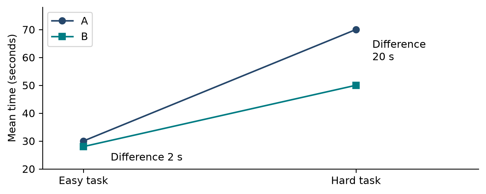
A factorial study manipulates more than one factor. Suppose an interface comparison is crossed with task difficulty. An interaction asks whether the interface difference depends on difficulty, rather than merely whether each factor has an average effect. Illustrative cell means are A easy 30, B easy 28, A hard 70, and B hard 50 seconds. The A−B difference grows from 2 to 20 seconds; the difference of differences is 18 seconds. These means alone do not provide an interaction p-value: replication and residual variation are still needed.
8 4 Repeated measures and alternative ANOVA models
When the same people use all three designs, ordinary independent-groups ANOVA is inappropriate. In a balanced one-factor repeated-measures analysis, total SS can be partitioned into condition, participant, and residual SS. Participant variation is removed from the denominator for testing condition. For n people and k conditions, condition degrees of freedom are k−1 and uncorrected residual degrees of freedom are (n−1)(k−1).
For more than two repeated conditions, the conventional univariate F test additionally relies on sphericity, equality of the variances of condition differences. Greenhouse–Geisser corrections adjust degrees of freedom when that assumption is questionable. Mixed-effects models provide another approach and can accommodate additional task and participant structure. Welch ANOVA addresses unequal variances in independent groups. None of these procedures fixes confounded assignment, ambiguous measurement, or informative missingness.
9 Regression correlation and models for HCI data
9 1 Correlation summarizes association
The sample covariance is the average product of centered values with divisor n−1. Pearson's correlation standardizes it by the two sample standard deviations:
Its range is −1 to 1 and it measures linear association. A value near zero can coexist with a strong curved relationship. A high value can be driven by an influential point, by mixing distinct populations, or by a confound. Scatterplots are essential. Spearman correlation applies Pearson's idea to ranks and is useful for monotonic relationships or ordered measurements, but it does not establish causation either.
Suppose frequent users finish quickly. Frequent use might build skill, but people who already find the interface easy might use it more, and professional role might explain both. Randomizing training can answer a causal training question; correlating observed usage with time cannot, on its own, distinguish those explanations.
9 2 Least squares and a worked slope
A simple linear model represents an outcome by a systematic component and an error:
Ordinary least squares chooses the intercept and slope to minimize SSE=Σ(yi−ŷi)². Setting the two derivatives of SSE to zero gives the normal equations; solving them yields
For a fictional five-person illustration, experience values are 1, 2, 3, 4, and 5 years, and task times are 12, 10, 9, 7, and 7 seconds. Here x̄=3, ȳ=9, Sxx=10, and Sxy=−13, so b₁=−1.3 seconds per year and b₀=12.9 seconds. The fitted line is ŷ=12.9−1.3x. At three years the fitted mean is 9 seconds. The intercept describes the extrapolated line at zero years; centering experience at three years would make the intercept refer to the middle of the observed data instead.
Residuals are .4, −.3, 0, −.7, and .6 seconds. SSE=1.10 and the residual variance estimate is s²e=SSE/(n−2)=.3667 seconds². Under independent normal errors with a correctly specified linear mean and constant variance,
This gives SE(b₁)≈.1915 and t≈−6.789 for testing a zero slope. The example is intentionally simple, and five invented observations cannot establish an empirical claim about expertise. In real data, the relationship might curve, task difficulty might differ with experience, and participants might have self-selected into their roles. A precise fitted slope does not remove those issues.
With an intercept in ordinary in-sample least squares, R²=1−SSE/SST. Here SST=18, so R²≈.939. This is the proportion of sample outcome variation accounted for by the fitted line relative to an intercept-only model. It is not the percentage of behavior caused by experience. High in-sample R² does not guarantee accurate prediction for new users; evaluate prediction on held-out data with splits that keep dependent records from the same participant together.
9 3 Confidence in a mean response and prediction of a person
For a predictor value x₀, the estimated standard error of the fitted mean response is
For a future individual's response, the prediction standard error adds 1 inside the square root. Prediction is more uncertain than estimating an average response, and uncertainty grows away from the center of observed x values. These formulas do not validate extrapolation outside the observed range. Bootstrapping a straight-line fit also does not turn a misspecified linear mean into a correct nonlinear model.
9 4 Multiple predictors and interactions
Regression generalizes group comparisons. Encode A as 0 and B as 1 in a model with an intercept: the coefficient of B is the B−A mean difference. With additional predictors, a linear model might be
where E is centered baseline experience. The interface effect is β₁+β₃E, so the interaction coefficient describes how the effect varies with experience. Centering makes β₁ the interface effect at a meaningful reference experience. In observational data, adding covariates does not guarantee elimination of confounding. In an experiment, well-chosen baseline covariates can improve precision; conditioning on a post-treatment variable can instead alter or bias the effect being estimated.
For multiple predictors, the least-squares solution is b=(XᵀX)⁻¹Xᵀy when the design matrix has full column rank. Under homoscedastic independent errors, its estimated covariance matrix is s²e(XᵀX)⁻¹, with residual degrees of freedom n−p for p fitted coefficients including the intercept. Highly correlated predictors make separate coefficients difficult to estimate. More predictors are not automatically better, especially in small HCI samples.
9 5 Binary counts and repeated observations
Linear models can predict impossible probabilities when used uncritically for binary data. Logistic regression models log odds:
Exponentiating β₁ gives an odds ratio for a one-unit predictor change, holding other modeled predictors fixed. It is not a risk ratio or a percentage-point change. At a baseline probability .10, doubling the odds gives probability .1818, not .20: baseline odds are .10/.90, doubled odds are .2222, and probability is .2222/(1+.2222). Report predicted probabilities or marginal differences when those are easier to interpret than odds.
Count models can use a log link, log(λi)=Xiβ+log(exposurei). The exposure term is an offset for differing opportunities, such as the number of tasks or interaction time. A Poisson model assumes conditional mean and variance are equal; overdispersion may motivate a negative-binomial model. Ordinal regression preserves the ordering of response categories without assuming equal intervals. Positive time outcomes may be modeled on a log scale or with an appropriate positive-valued distribution.
For repeated trials, a mixed model can include participant and task effects:
Here ui is a participant-specific intercept and vj a task-specific intercept. Random slopes can allow the interface effect to vary across participants. This model retains trials while acknowledging dependence and variation across sampled tasks. Its assumptions, convergence, and complexity still need checking; fitting a complex model to very few people does not manufacture information. In human–AI evaluation, outputs may also vary across model versions, prompts, and stochastic generations. Model or control those sources of variation rather than counting every model response as an independent human participant.
10 Power and sample size planning
10 1 Three different reasons for choosing n
Discovery, precision, and hypothesis testing require different calculations. A study intended to find usability problems asks how likely it is to encounter them. A benchmarking study may target an interval width. A comparative experiment may target power for a specified effect. “How many users for p<.05?” has no unique answer, and no finite n guarantees significance for an unknown true effect. Sample-size justification should identify the objective, effect or precision target, assumptions, and constraints. [R6]
For discovering one particular problem that each independent relevant participant encounters with probability q, the probability of observing it at least once is
For q=.30, five participants give .8319 and eight give .9424. For q=.05, five give only .2262. To reach a target discovery probability γ, solve
Round up: with q=.30 and γ=.90, n≥6.456, so seven participants are needed. This calculation concerns one problem with the stipulated exposure probability, not a guarantee to discover 90% of all flaws. Real problems differ in probability, tasks expose different opportunities, and user groups differ. The formula explains diminishing returns for repeated encounters with common problems; it is not a universal five-user rule and is not a t-test power calculation.
10 2 Type II error and a specified alternative
Type I error is rejecting a true null. Type II error, β, is failing to reject under a specified alternative. Power is 1−β. It depends on the true effect, noise, sample size, test, alpha, design, and decision rule. A study with 80% power for a 5-second difference may have poor power for a 1-second difference. “80% chance of detecting any real effect” omits the condition that makes the statement meaningful.
For a roughly normal standardized statistic under an alternative, let λ be the effect divided by its standard error. With two-sided critical value zc=z1−α/2, approximate power is
The alternative distribution shifts away from the null, increasing the chance of crossing either critical boundary. Higher target power and smaller alpha generally require larger samples, but the relationship is not a simple direct proportion. The effect-size dependence is approximately inverse square when other quantities remain fixed: halving the target difference often requires about four times as many observations, not an exponential increase.
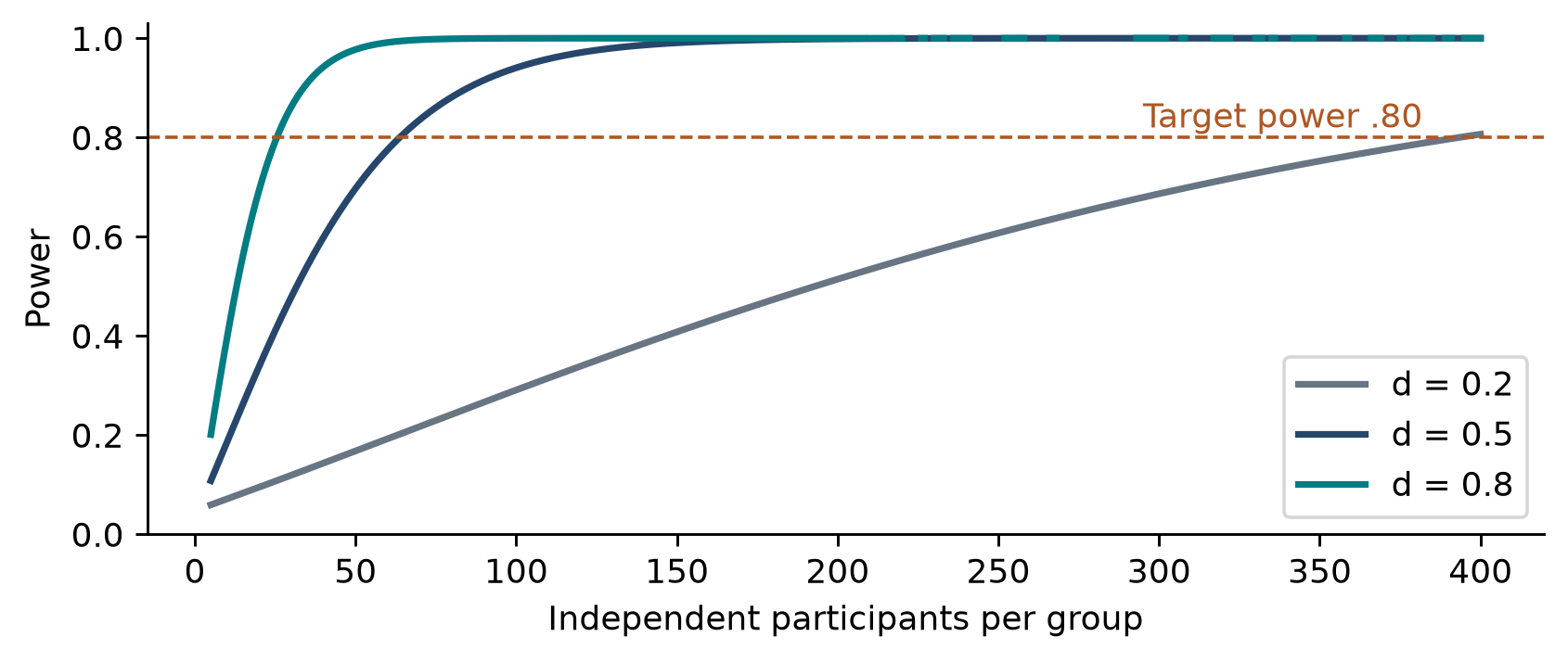
10 3 Mean differences and precision targets
For two equally sized independent groups with anticipated common SD σ and target difference δ, a normal approximation gives per-group size
With σ=10 seconds, δ=5 seconds, α=.05, and power=.80, n≈2×100×(1.960+.842)²/25≈62.79 per group. Round up to 63 for this approximation; a calculation using the noncentral t distribution requires 64 per group. The total is then 128. Distinguish per-group n from total N whenever reporting a calculation.
For paired observations, replace the independent-group noise with the anticipated SD of differences σd:
With δ/σd=.5, the approximation is about 31.4 paired participants, rounded to 32; noncentral t planning gives 34. This reduction is meaningful only if the assumed difference variability and paired design are credible. Obtain planning values from relevant prior evidence, a range of plausible scenarios, or a pilot interpreted with its uncertainty. A tiny pilot's observed effect is a fragile basis for recruitment.
For a mean with desired approximate confidence-interval half-width h and known planning SD σ, n≈(z1−α/2σ/h)². With σ=12 seconds and h=3 seconds, n≈61.47, rounded to 62 under the normal approximation. For a proportion with half-width h, the corresponding approximation is n≈z²π(1−π)/h²; using π=.5 gives a conservative maximum variance when the rate is unknown. These are precision calculations, not promises about p-values.
10 4 Power for two proportions
A change from .10 to .12 is a two-percentage-point improvement. For independent arms with equal n, a widely used normal approximation is
Using α=.05, power=.80, πA=.10, and πB=.12 gives approximately 3840.85 users per arm, rounded up to 3,841, or 7,682 total. The two square-root terms account separately for null and alternative variability. A simpler approximation that combines the z values before multiplying by the unpooled variance gives a nearby but different number. Software can also differ through continuity corrections, exact versus asymptotic tests, or power definitions; report the procedure and inputs. R's power.prop.test documentation explicitly identifies n as the number per group. [R7]
| Baseline | Target rate | Absolute improvement | Approximate n per arm | Total after rounding |
|---|---|---|---|---|
| .10 | .11 | 1 percentage point | 14,751 | 29,502 |
| .10 | .12 | 2 percentage points | 3,841 | 7,682 |
| .10 | .15 | 5 percentage points | 686 | 1,372 |
Small online effects can demand thousands of independent users even though a laboratory comparison of a large time effect may require dozens. A fixed “20–30 participants” recommendation cannot cover both. The unit still matters: many visits from one user may not equal many independent users. Plan follow-up duration to observe the outcome and relevant temporal patterns; no universal number of business cycles eliminates novelty effects.
10 5 What sits behind an F power table
For balanced one-way ANOVA with k groups, common within-group SD σ, and specified population means μj, define Cohen's f using the average squared separation of group means:
Under the alternative, the test statistic has a noncentral F distribution with degrees of freedom k−1 and N−k and noncentrality λ. For a candidate N, find the upper-alpha critical value Fc from the central F distribution, then calculate
Increase N until the target power is reached, retaining balanced group sizes if required. For k=3, f=.25, α=.05, and power=.80, the smallest balanced solution is 53 per group, N=159. The number of measured outcomes does not replace the effect-size and variance inputs. Repeated-measures ANOVA additionally needs assumptions about correlations and sphericity; interaction power requires the particular interaction effect rather than only a main-effect size.
10 6 Feasibility attrition and sensitivity
If 64 usable participants per arm are needed and 10% loss is anticipated, recruiting ceil(64/.90)=72 per arm is a simple planning adjustment. It protects expected count, not validity: differential attrition related to condition or outcome still needs analysis. Account for multiple confirmatory outcomes, clusters, exclusions, and unequal allocation when they are part of the design.
If resources cap n, conduct a sensitivity analysis: report the effects the planned study can detect or the precision it can achieve. A constrained study can still be informative, but its claims must match its sensitivity. After collecting data, “observed power” obtained by substituting the observed effect usually restates the p-value and adds little. Report the effect and interval, and use external or substantively meaningful effects for future planning.
11 Bootstrapping and randomization inference
11 1 What a bootstrap sample actually contains
The ordinary nonparametric bootstrap approximates the population distribution by the empirical distribution, which assigns probability 1/n to each observed case. It draws n cases with replacement and recalculates the statistic. Repeat that process R times to obtain a bootstrap distribution of the estimator. Sampling with replacement means one observed participant may appear multiple times in a resample while another does not appear. It does not mean inventing values between observed points or appending synthetic users to the original study.
With the three observations [1,2,9], the original mean is 4. A resample [1,1,2] has mean 1.333; [9,2,9] has mean 6.667. Variation comes from how often observations are selected. These are a demonstration of mechanics, not a reliable population analysis from three cases. If the three observations were all 4, every bootstrap mean would also be 4, yielding a misleadingly narrow picture if the sample omitted real population variation. Tiny samples do not necessarily produce visibly wide intervals.
With n=30 and R=10,000, generate 10,000 separate samples, each containing 30 draws. There are 300,000 selections but still only 30 observed participants. Increasing R reduces numerical Monte Carlo error in the resampling approximation. It does not increase the information about unobserved people and does not force the bootstrap distribution to be normal. [R8]
11 2 Standard error and percentile intervals
Let θ̂ be the statistic from the original data and θ̂*r its value in bootstrap replication r. The bootstrap standard error is the sample standard deviation of those R statistics:
Do not divide this standard deviation by √R when estimating sampling uncertainty of θ̂. Doing so estimates Monte Carlo precision of a simulation average and makes apparent uncertainty shrink merely because the computer runs longer. Likewise, do not submit 10,000 bootstrap means to an ordinary independent-sample t test as though they were 10,000 recruited users.
The percentile interval takes quantiles of the bootstrap statistics:
At R=10,000 these cutoffs are near ordered positions 250 and 9,750; exact indexing and interpolation depend on the quantile convention. Software should compute the quantiles. Do not discard actual participants, and do not average the central 9,500 bootstrap statistics to obtain the interval. Report the original point estimate and the two endpoints. Bias-corrected and accelerated intervals, studentized intervals, and other bootstrap procedures have different constructions and performance; “bootstrap CI” alone is incomplete reporting.
11 3 Preserve pairing and compare the actual contrast
For the booking study, resample twelve participant pairs, or equivalently resample the twelve paired differences. A participant's A and B observations must travel together. Compute the mean difference in each replication. For two independent arms, resample within each arm separately at its original sample size and calculate the difference of means in each replication. Repeated-trial studies generally require resampling participants or another appropriate cluster, not individual dependent trial rows.
The contrast distribution is the object of interest. Do not independently sort the two lists of bootstrap means and subtract matching ranks: that invents a dependence structure. Subtract the estimates within each replication, then take quantiles of the resulting differences. There is no need to wait for overlapping arm-specific intervals before analyzing the contrast; it is the direct analysis from the beginning.
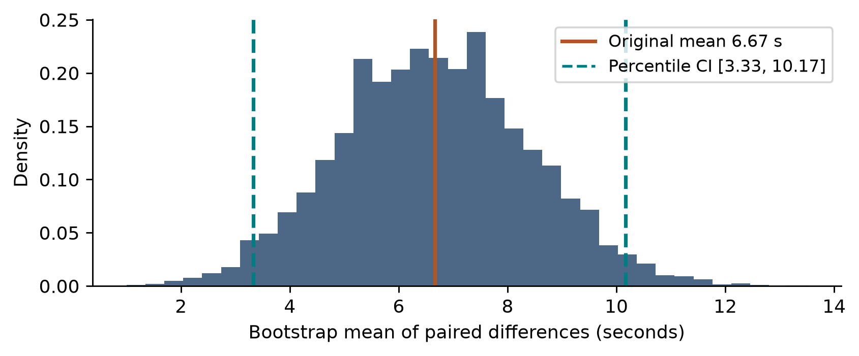
For this particular computation, the bootstrap SE is about 1.744 seconds and the percentile interval is [3.33,10.17] seconds. The original estimate remains 6.67 seconds. The interval differs from the paired t interval [2.65,10.68] because the procedures approximate uncertainty differently. Its narrower width is not evidence that it is more accurate; a twelve-person empirical distribution and an uncorrected percentile method can have limited coverage accuracy.
Separate 95% intervals for A and B can overlap even when a valid interval for their difference excludes zero, particularly with positive within-person correlation. Substantial overlap is not proof of equivalence. If the contrast interval includes zero, it expresses uncertainty about the contrast; it does not establish a tie or supply an automatic decision to retain or deploy an interface.
11 4 When resampling helps and when it does not
Bootstrapping is useful when the sampling distribution of a statistic is awkward to derive, such as some medians, trimmed means, ratios, or complex contrasts. It can be used alongside parametric analysis rather than only after a normality test “fails.” Unequal variances alone do not make it necessary: Welch's test directly addresses that issue. Skew does not automatically invalidate every t procedure, and multimodality does not make a mean undefined.
The bootstrap still needs the observed data and resampling scheme to approximate the relevant sampling process. It cannot recover an absent user population, repair confounding, undo a biased exclusion rule, or reliably estimate an unobserved rare tail from a tiny sample. Some statistics, boundary cases, extreme quantiles, and dependent processes need specialized methods. A percentile interval can have poor coverage when bias or skew is substantial; selecting a bootstrap method is part of the analysis, not an automatic guarantee of validity. [R8; R9]
11 5 A randomization test asks a different question
Bootstrap resampling approximates estimator uncertainty around the observed empirical distribution. A randomization test creates a null reference distribution by reallocating labels according to the actual randomization scheme. For a valid independent-group randomized study under a sharp no-effect null, retain outcomes, repeatedly reassign the allowed group labels, and recalculate the contrast. For an appropriate paired design, permitted within-pair swaps correspond to changing difference signs. Restrictions such as blocks or clusters must be retained.
For R randomly drawn null reallocations, a common Monte Carlo p-value is (1+b)/(R+1), where b counts simulated statistics at least as extreme as the observed statistic. For exhaustive enumeration of all allowed allocations including the observed one, use the exact fraction of extreme allocations. A generic permutation assumes the required exchangeability; arbitrary shuffling is not universally valid for every weak null, unequal-variance setting, or time series.
A bootstrap distribution centered near the observed effect is not automatically a null distribution. The proportion of its values above or below zero is not a generic exact p-value. Bootstrap hypothesis tests exist, including null-centered and studentized constructions, but their assumptions and target differ from simply calculating a percentile interval. The method should follow the question rather than the available button in software.
12 Robust analyses ordinal data and transformations
12 1 Diagnose the model rather than hunt for a passing test
Start with plots that expose raw values and design structure. Use paired lines for matched observations, dot plots or empirical cumulative distributions for independent groups, and residual-versus-fitted and quantile–quantile plots for models. Check data-entry errors and timing boundaries before statistical diagnostics. A normality test has little sensitivity in tiny samples and can detect negligible departures in huge samples; its p-value should not be the sole method-selection rule.
A quantile–quantile plot compares ordered residuals or relevant differences with theoretical normal quantiles. Curvature or isolated points may identify skew, heavy tails, or influence. Residual patterns against predicted values may indicate a nonlinear mean or changing variance. Independence usually comes from the study structure and cannot be certified by an ordinary residual histogram. Choose remedies for the problem actually present: Welch for independent unequal variances, a suitable mean model for nonlinearity, and clustered or multilevel inference for dependence.
For positive times, a log transform often makes multiplicative differences easier to model. If ℓᵢ=log(Aᵢ)−log(Bᵢ), a paired analysis of ℓ estimates the mean log ratio. Exponentiating its estimate and interval gives a ratio of geometric means. A ratio 1.20 means the geometric mean time for A is 20% higher than B; it does not say that the arithmetic mean difference is 20%. A transform changes the estimand. Explain that change and do not log zeros by adding an arbitrary constant without justification.
12 2 Rank and sign procedures
The paired sign test asks whether a positive difference is as likely as a negative one, conditional on the treatment of zeros. It ignores magnitudes. In the booking dataset, nine differences are positive, two are negative, and one is zero. Omitting the zero, the exact two-sided binomial sign test is about .0654. This differs from the paired t result because the sign test asks a different question and uses less information, not because one computation must be wrong.
The Wilcoxon signed-rank procedure ranks absolute nonzero differences and sums ranks by sign. For a location-shift interpretation it relies on symmetry of the difference distribution, in addition to independent pairs. Ties and zeros affect calculations. The Mann–Whitney procedure ranks independent groups; one useful effect interpretation concerns the probability that a random observation from one group exceeds one from the other, with half weight for ties. It is not simply a general-purpose test of medians unless additional distributional assumptions hold.
Kruskal–Wallis extends independent-group rank comparison to several groups, while Friedman addresses a complete blocked or repeated-measures structure. Significant omnibus results still need appropriate follow-up contrasts and multiplicity handling. Aligned rank transform methods can support some factorial questions, but their alignment and contrast procedures matter. Nonparametric does not mean assumption-free, and transforming everything to ranks can discard scientifically important differences in seconds or error counts. Wobbrock and Kay provide a dedicated HCI treatment of these choices. [R13]
12 3 Outliers and robust estimators
An extreme completion time can be a logging error, an interruption, a misunderstanding, or a genuine design failure. Those explanations have different consequences. Correct demonstrable errors while retaining an audit trail. Apply prespecified exclusion rules consistently. Report sensitivity to reasonable alternatives when an influential observation materially changes the conclusion. Deleting a difficult participant because significance improves is not a defensible cleaning rule.
A trimmed mean removes a specified fraction from each tail before averaging and targets a different location summary from the ordinary mean. Robust estimators can reduce sensitivity to extreme values, but an extreme usability failure may be the outcome that matters most. Report tail behavior or failures explicitly instead of making them disappear from the design discussion. Robustness of inference and importance of rare harms are separate concerns.
13 Online experiments missing data and repeated decisions
13 1 Stable assignment and meaningful outcomes
A web experiment should assign eligible users consistently to concurrent variants, preserve assignment across repeated visits when that is the intended unit, and log both assignment and exposure. Before interpreting outcomes, inspect instrumentation, eligibility, and denominators. Clicking a button is not the same outcome as completing the transaction behind it. A more conspicuous button can increase accidental clicks while reducing successful bookings.
Define a primary outcome linked to the research question and a limited set of guardrail outcomes such as failures, abandonment, or accessibility problems. Guardrails are not decorative: explain how adverse evidence affects interpretation. If one user's treatment changes another user's experience, as in a collaborative workspace, the no-interference assumption of a simple user-level A/B model may fail. Assignment and analysis may need to occur at team, classroom, or organization level.
An A/A test compares randomized groups receiving the same interface. It can reveal allocation or measurement problems, but a correctly calibrated .05 test will still occasionally reject by chance. One A/A result does not prove or disprove the entire pipeline. Repeated calibration, logs, and engineering checks provide stronger evidence than a single threshold.
13 2 Sample ratio mismatch is a diagnostic signal
If intended allocation is 50:50 but observed counts are 10,000 and 9,500, expected counts are 9,750 each. The Pearson goodness-of-fit statistic is
With one degree of freedom, the approximate p-value is .000343. That is strong evidence against the simple allocation model, not logical proof of a particular bug. An unexpectedly imbalanced count may reflect assignment, exposure logging, eligibility filters, or outcome-dependent losses. Planned unequal randomization is not itself a mismatch; compare with the specified ratio. [R14]
Removing 500 observations from the larger arm makes the counts equal but does not restore users lost selectively from the other arm. Investigate the cause and document any recovery or reanalysis. Random thinning does not inherently make every variance calculation invalid, but it wastes information and does not repair selection bias. Whether a study can be salvaged depends on the identified mechanism and recoverable records, not a blanket rule that every imbalance is either harmless or irreparable.
13 3 Missingness depends on what is observed
Missing completely at random, or MCAR, means that missingness is independent of both observed and unobserved values in the model. Missing at random, or MAR, means that after conditioning on relevant observed information, missingness does not depend on the missing values. MAR can depend on treatment and measured covariates; it does not mean that missingness has no relation to the experiment. Missing not at random, or MNAR, means dependence on unobserved values remains after conditioning on observed information.
For example, questionnaire response might depend on recorded device type and assigned interface. A suitable MAR analysis might condition on those variables if they make remaining missingness independent of the unobserved rating. If people with extremely low unrecorded satisfaction are more likely to omit the rating even within those categories, MNAR is plausible. These assumptions are generally not fully testable from the observed data alone.
Complete-case analysis, multiple imputation, weighting, and explicit missingness models address different assumptions. Multiple imputation creates several plausible completed datasets under a model and combines estimates and uncertainty; it is not simply replacing every missing value with one prediction. Sensitivity analyses should examine conclusions under plausible departures from the assumed mechanism. A known server outage does not automatically establish MCAR if it affected a particular time period or device group.
Abandonment may itself be an observed outcome rather than a record to discard. Analyze assigned participants according to a prespecified treatment-policy or intention-to-treat estimand when appropriate, and distinguish that from an analysis limited to actual exposure or protocol completion. Neither label solves unobserved outcomes by itself. Record why data are absent and show participant flow from eligibility through analysis.
13 4 Peeking multiplicity and preregistration
Repeatedly checking a fixed-sample p-value and stopping when it first crosses .05 changes the procedure's Type I error rate. The amount of inflation depends on the monitoring and stopping rule; it is not universally 30%. Valid group-sequential designs, alpha-spending procedures, and other sequential methods explicitly account for monitoring. A fixed-sample plan instead specifies its target and stopping rule in advance, apart from necessary ethical or operational stops.
Multiplicity also arises from many outcomes, subgroup analyses, task definitions, time windows, and alternative exclusion rules. A prespecified primary analysis makes the central claim easier to assess. Exploratory analyses are valuable when labeled as such and followed by suitable validation. A preregistration should state hypotheses, estimands, recruitment and stopping, outcomes, exclusions, statistical models, planned contrasts, and how missing data will be handled. Record deviations rather than pretending the plan never changed.
Longer duration can expose temporal variation, but novelty effects and learning have no universal expiration date. If long-term adoption is the research question, observe the relevant horizon or design a longitudinal study. Pooling early and late behavior may conceal the very interaction with time that matters.
14 Equivalence Bayesian estimation and practical decisions
14 1 Evidence for a small enough difference
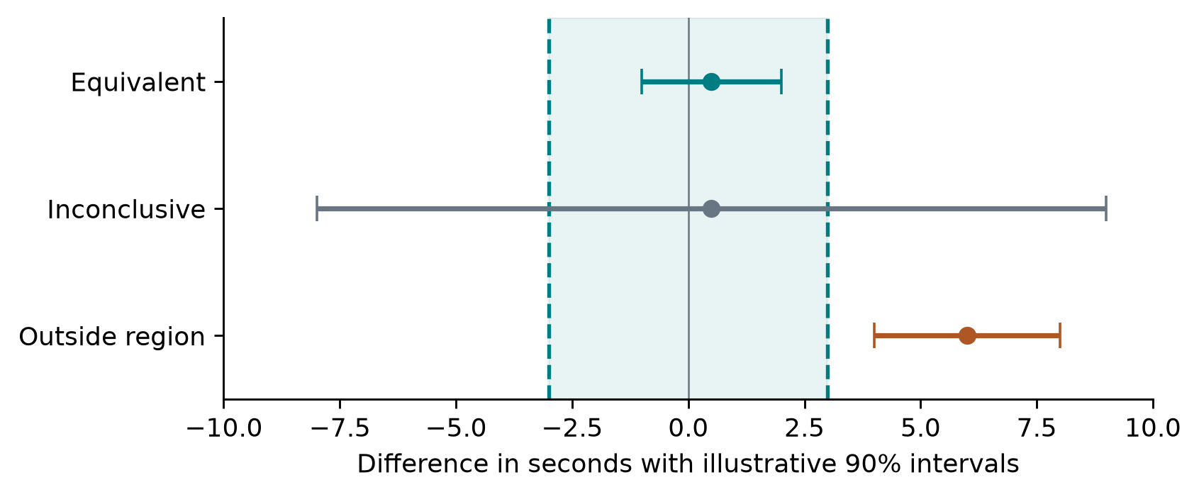
Suppose two booking interfaces differ in appearance, and the research question is whether their mean times are practically equivalent within ±3 seconds. An ordinary test of Δ=0 cannot establish equivalence merely by yielding p>.05. The equivalence hypotheses instead place the unacceptable region in the null:
The two one-sided tests procedure, TOST, rejects both parts of the null at a chosen α. For the usual matching procedures at α=.05, equivalence is supported when the 90% confidence interval falls entirely within prespecified bounds. A 95% interval is used for the ordinary two-sided .05 zero-effect test, so the different confidence level is intentional. Bounds must be justified by task consequences or theory, not chosen after seeing the data. [R15]
An estimate can be statistically distinguishable from zero and still small enough to be equivalent for practical purposes. Conversely, an imprecise result can support neither a difference nor equivalence. Noninferiority asks a related one-sided question: can an unacceptable disadvantage be ruled out? It needs a justified margin and a design capable of addressing that claim.
14 2 A Bayesian interval uses an explicit probability model
Bayesian analysis combines a prior distribution for a parameter with the likelihood of observed data. The posterior is proportional to likelihood times prior:
A credible interval contains a specified posterior probability under that model. This is different from frequentist repeated-sample coverage. A prior is not an embarrassment to hide: document it, explain its scale, and examine sensitivity when it materially affects the answer. Bayesian inference also does not fix biased recruitment, confounded assignment, or incorrect likelihood assumptions.
For a transparent binary example, use a Beta(a,b) prior for success probability π and observe x successes in n independent Bernoulli trials. The posterior is Beta(a+x,b+n−x). With a uniform Beta(1,1) prior and 18 successes out of 20, it becomes Beta(19,3), whose mean is 19/22≈.864. Equal-tail credible endpoints come from its .025 and .975 quantiles. The estimate differs from the raw .90 because the prior contributes information. A different defensible prior can yield a different posterior, particularly with small n.
For an HCI comparison, a posterior probability such as P(Δ>5 seconds|data) directly addresses a specified practical threshold, provided the model is appropriate. It is not obtained by subtracting a frequentist p-value from one. Bayes factors compare models through marginal likelihoods and can be sensitive to prior choices; they are not confidence intervals in another form.
14 3 A research conclusion is more than a test decision
Use the evidence to answer the operational question. Is the likely improvement large enough to matter? Are harmful outcomes sufficiently constrained? Which populations and tasks were actually studied? Do interviews or observations suggest an explanation that the numerical outcome alone cannot establish? A click-rate increase does not demonstrate comprehension, and a time reduction does not demonstrate accessibility.
The statistical interval addresses selected sources of uncertainty under a model. It generally does not include unknown logging bias, unmeasured confounding, or the uncertainty of transferring from a classroom task to everyday work. State those limitations directly. Product choices may also depend on implementation cost, reversibility, user preference, and alternatives; a threshold crossing is not an instruction to deploy.
15 AI and machine learning for analyzing experimental data
15 1 Choose the analytical question before the algorithm
An HCI experiment can produce thousands of clicks, gaze samples, utterances, and screen recordings from a modest number of people. Machine learning can help turn these records into predictions, behavioral descriptions, and measurements that are difficult to obtain manually. The researcher still has to decide what each output means and how its accuracy will be established. More recorded rows do not create more independent participants.
Consider three questions about a booking experiment. “Does interface B reduce failure?” asks for an experimental effect. “Can early pauses and errors predict eventual failure?” asks for predictive performance on new observations. “Which navigation strategies recur in the logs?” asks for exploratory structure. These questions can use the same dataset but require different validation. Predictive success does not establish that changing an influential feature will change the outcome. A cluster is a discovered description, not automatically a population category or causal explanation.
Statistics and machine learning overlap substantially. Logistic regression is both a statistical model and a supervised learning algorithm. The useful distinction here is the analytical target: estimating an effect with uncertainty, predicting an unseen outcome, discovering structure, or constructing a measurement from raw material. The method must serve that target. A flexible algorithm cannot compensate for an undefined outcome or an unsuitable sample.
| Analytical task | HCI example | Evidence needed |
|---|---|---|
| Supervised prediction | Predict task failure from early interaction | Performance on appropriately held-out people or sessions |
| Unsupervised exploration | Discover recurring navigation strategies | Stability, source-record inspection, and replication |
| Automated measurement | Code confusion in think-aloud excerpts | Agreement and error analysis against independent human judgments |
| Signal representation | Extract gaze or movement features | Valid sensor processing and correspondence to the intended construct |
15 2 Define the observation and prediction time
Let xᵢ be the feature vector for an observation and yᵢ its recorded outcome. Supervised learning estimates a function f(xᵢ) from labeled training data. For a binary outcome, yᵢ=1 might mean task failure and f(xᵢ) might estimate its probability. Specify both the unit and the moment at which the prediction is made. A model that predicts failure after thirty seconds can use only information available by that point. Final completion time, an error recorded after abandonment, or the evaluator's final success code would leak future or target information.
Define eligibility too. If prediction occurs at thirty seconds, does the dataset include only tasks still in progress then? Excluding already completed tasks changes the target population. An alternative is prediction at a defined interaction milestone. In either case, document the risk set, outcome horizon, treatment of early completion, and missing observations. A retrospective detector that labels an entire completed session is legitimate, but it answers a different question from an early-warning model.
Identifiers organize the analysis rather than automatically belonging among predictors. Keep participant, session, task, device, and condition identifiers so records can be split and errors investigated. A participant identifier may allow memorization without helping on a new person. A task identifier can similarly make results depend on seeing the same task during training. For a small study, begin with a few substantively justified features and a simple baseline; thousands of engineered variables can overwhelm the available independent evidence.
15 3 Validation must preserve the study structure
A random row split can put one person's trials in both training and testing. If the intended claim concerns new users, the test then gives the model familiarity with the very people it should encounter as strangers. Keep all records of a participant in one partition. Grouped cross-validation rotates held-out participant groups. A split by session, task, organization, or time may instead be required by the intended application. The scikit-learn cross-validation guide documents group-aware splitting. [R16]
For prediction on unseen tasks as well as unseen people, holding out only people is insufficient. Consider a separate task holdout or a design that excludes both relevant sets from training; its smaller effective training set is part of the cost of testing that broader claim. For future sessions of known users, a temporal split can be appropriate, but avoid training on later records to predict earlier ones. Overlapping signal windows also need separation at their originating recording or session, with a time buffer where appropriate.
Preprocessing belongs inside the training procedure. Estimate means, standard deviations, imputation rules, selected features, and learned representations from the current training subset. Apply those fixed transformations to its validation subset. A pipeline helps enforce this boundary. It does not choose the correct split or recognize a feature that directly encodes the answer. [R17]
Hyperparameter tuning needs another boundary. In nested cross-validation, each outer split estimates the performance of the full model-selection procedure. Only its training portion enters an inner cross-validation loop that chooses regularization strength, tree depth, or other settings. The outer held-out portion is used after those choices. If an independent final test set is also reserved, lock the models and decision rules before examining it. Selecting the best reported test score among many attempts turns that test into another development set. [R18]
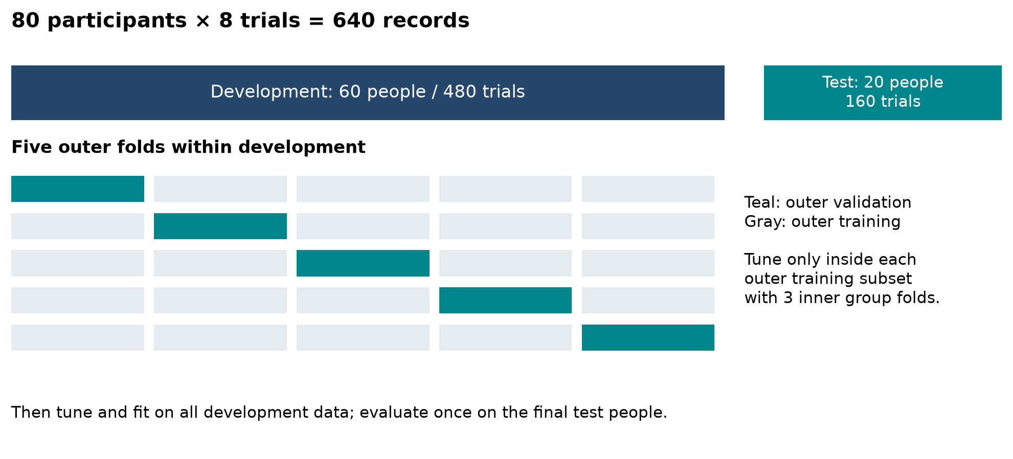
15 4 Two models and the mathematics of fitting
Logistic regression connects a linear score to a probability. With p features and coefficients β, write
For an illustrative score η=−2+0.3×pause+0.6×errors+0.5×hard, a pause of four seconds, two errors, and hard=1 give η=0.9 and predicted probability about 0.711. These coefficients are chosen solely to illustrate the calculation; they are not the fitted coefficients of the later simulation. A threshold of 0.5 would classify this observation as likely failure.
Fitting minimizes a loss that penalizes inaccurate probabilities. One convention for penalized logistic regression is
The first term is average binary log loss; the second shrinks coefficients to reduce excessive fitting. Here the intercept is unpenalized. The penalty trades training fit against model complexity. Its numerical scale depends on software conventions: scikit-learn's C controls inverse regularization strength, so larger C means weaker regularization, but it should not be read as an exact reciprocal of λ in every displayed loss convention. Standardizing predictors using training-only statistics makes coefficient penalties more comparable across measurement units. [R19]
A decision tree divides the feature space with questions such as “were there at least two errors?” or “was the pause longer than six seconds?” A leaf predicts from its training observations. With binary classes and failure proportion q in a node, Gini impurity is
A split reduces impurity by G(parent)−[NₗG(left)+NᵣG(right)]/N. For ten failures and ten successes, parent impurity is 0.5. Suppose a split creates a ten-observation leaf with eight failures and a ten-observation leaf with two failures. Each child has impurity 0.32, so the reduction is 0.18. Repeated splits can represent nonlinear relationships and interactions, but deep trees can fit peculiarities of a small sample. Maximum depth and minimum leaf size constrain that flexibility. [R20]
Random forests and boosted trees offer other ways to combine nonlinear rules. Greater complexity should earn its place through validation against the baseline. The central requirement is not that a method be called AI; it is that the resulting analysis answers the question reliably.
15 5 Worked example of predicting task failure
The following fully fictional simulation contains eighty participants with eight trials each. Features represent pause duration and error count observed during a defined early interaction window, plus a task-difficulty indicator. The outcome is eventual failure. A latent participant characteristic affects both observed behavior and failure, creating dependence among one person's trials. This is a methodological illustration rather than a realistic model of all booking behavior.
Sixty participants supply 480 development trials. Twenty different participants supply 160 final test trials. Participant identifiers are used for splitting but excluded from the predictor matrix. Five outer participant folds evaluate each tuning procedure; three inner participant folds select C from {0.1,1,10} for logistic regression and maximum depth from {2,3,4} for a tree with minimum leaf size eight. Both use mean log loss for selection. Feature scaling is inside the logistic pipeline. The final models are tuned on all development participants with five grouped folds and then fitted to all development data.
The baseline gives every observation the development-set failure rate. For classification, all three models use the prespecified threshold 0.5. This baseline tests whether the features add useful information beyond knowing the overall event frequency. A classifier that always predicts success can have high accuracy when failure is rare, while detecting no failures at all.
The development set contains 171 failures (35.625%); the test set contains 55 (34.375%). The pooled outer-fold log losses are 0.544 for logistic regression and 0.609 for the tree. Final tuning selects C=1 and tree depth two. The locked test results are:
| Metric | Baseline | Logistic | Tree |
|---|---|---|---|
| Accuracy | 0.656 | 0.756 | 0.738 |
| Precision | Undefined | 0.690 | 0.659 |
| Recall | 0.000 | 0.527 | 0.491 |
| F1 | 0.000 | 0.598 | 0.562 |
| ROC AUC | 0.500 | 0.812 | 0.766 |
| Average precision | 0.344 | 0.722 | 0.581 |
| Brier loss | 0.226 | 0.161 | 0.176 |
| Log loss | 0.644 | 0.489 | 0.530 |
These numbers demonstrate the analysis workflow. The simulation mechanism uses a logistic relationship and therefore favors some model assumptions; it cannot establish that logistic regression generally outperforms trees in HCI. Development cross-validation and the final test also evaluate fits trained on different numbers of participants. A difference between their scores is not automatically evidence of leakage or a software error.
15 6 Read the confusion matrix and probability metrics
Take failure as the positive outcome. TP counts failures correctly flagged, FP counts successful trials incorrectly flagged, FN counts missed failures, and TN counts successful trials correctly left unflagged. The matrix needs named axes: confusing true and predicted labels swaps the meaning of precision and recall.
For the logistic model, the 160 held-out trials give:
| Actual result | Predicted success | Predicted failure |
|---|---|---|
| Success | TN = 92 | FP = 13 |
| Failure | FN = 26 | TP = 29 |
Thus precision is 29/(29+13)=0.690, recall is 29/55=0.527, and F1 is 58/(58+13+26)=0.598. Accuracy is 121/160=0.756, but the model still misses 26 of the 55 failures. Whether this is adequate depends on the intended use and error costs.
Accuracy is (TP+TN)/N, while specificity is TN/(TN+FP). When a method predicts no positive cases, precision is undefined; some software reports zero by convention. Report that convention rather than interpreting the zero as an observed fraction. Macro-averaged metrics give classes equal weight; micro-averaged metrics aggregate decisions. State the averaging rule for multiclass or multilabel outcomes. [R21]
Changing the threshold trades missed failures against false alerts. ROC curves plot recall against false-positive rate across thresholds; ROC AUC measures ranking discrimination. Precision–recall summaries are often informative for rare failures because precision exposes the false-alert burden. Average precision summarizes precision as recall increases; it depends on the event prevalence and is not numerically identical to every trapezoidal PR-area calculation. Choose the metric and operating threshold from the research purpose and development evidence, not by maximizing the final test result.
Probabilities need evaluation too. The binary Brier score averages squared probability error:
A predicted probability of 0.8 contributes 0.04 if failure occurs and 0.64 if it does not. Lower average loss is better. Log loss also assesses probabilities and penalizes confident mistakes strongly. Calibration asks whether events occur approximately 70% of the time among predictions near 0.7. A reliability diagram compares observed frequencies with predicted probabilities, with counts and uncertainty in each bin. Neither good ranking nor a lower Brier score alone proves good calibration. Any recalibration must be learned without using the final test outcomes. [R22]
If false alerts have cost C_FP and missed failures cost C_FN, with zero cost for correct decisions and calibrated probabilities, flagging is optimal under this simple cost model when π>C_FP/(C_FP+C_FN). For costs one and four, that threshold is 0.2. Real interventions can alter outcomes, consume staff time, or annoy users, so prediction accuracy alone does not establish the benefit of deploying the alert.
15 7 Quantify uncertainty in predictive comparisons
Evaluate competing models on the same held-out observations and compare paired losses. For tree prediction tᵢ and logistic prediction ℓᵢ, define
A positive Δ favors logistic regression on Brier loss. Because trials are clustered within people, resample held-out participants with all their trials, retaining both models' predictions for each record. In this balanced example, averaging within each participant and bootstrapping those twenty participant means gives the same point estimate as averaging the 160 trial losses. With unequal trial counts, an average-person target and an average-trial target generally differ; choose the weighting deliberately.
In the example, the observed tree-minus-logistic Brier difference is 0.01505. A paired participant bootstrap with 10,000 resamples and seed 567 gives a percentile 95% interval of approximately [0.00237, 0.02926]. Under this resampling analysis, the fitted logistic model has lower expected loss for the sampled test population. The magnitude and its practical value matter alongside the interval; this is not a universal ranking of the algorithms.
This interval concerns test-population sampling for these fixed fitted models. It does not include the variability of obtaining a different training sample and refitting or reselecting the models. Repeated studies or a carefully designed resampling procedure that repeats the entire training pipeline address that additional target. Twenty independent test participants still provide limited evidence even though the table has 160 rows. Ordinary binomial intervals treating all trial decisions as independent can be misleading.
Cross-validation folds share much of their training data. Their scores are not independent replications, so dividing the fold-score SD by √K and treating it as an ordinary standard error is generally unjustified. Report the splitting procedure and participant counts, inspect performance across folds, and distinguish a descriptive fold spread from a calibrated confidence interval. [R26] A single high score should also be checked for subgroup failures, device dependence, and deterioration on a new task or session.
15 8 Clustering and representations reveal candidate patterns
Suppose each session is summarized by standardized pause duration, number of backtracks, fraction of direct navigation, and help requests. K-means chooses cluster assignments cᵢ and centers μₖ to minimize within-cluster squared distance:
The algorithm alternates assigning observations to nearby centers and recomputing those centers. Changing feature scales changes distances and therefore the resulting groups. K must be chosen, and a low objective value does not show that there are K natural kinds of user. Examine sensitivity to K, feature choices, initialization, and participant resampling. A silhouette score compares within-cluster cohesion with separation from other clusters; it evaluates a geometric property, not the substantive truth of a persona. [R23]
For HCI interpretation, reopen representative and boundary cases in the logs or recordings. A cluster with many pauses could reflect planning, distraction, motor difficulty, or a logging failure. Name it descriptively before assigning a psychological explanation. If clustering used task time, testing whether the discovered clusters differ in task time on those same observations is circular confirmation. Freeze the representation and assignment procedure, then assess predictions or external variables on new data where possible.
Dimensionality reduction compresses features into a smaller representation. PCA retains directions of high variance, which need not be the directions most relevant to usability. Text embeddings can group semantically similar comments, but proximity in an embedding space does not validate a thematic interpretation. A visually separated two-dimensional projection is a prompt for investigation, not proof of stable populations.
15 9 Signals and automated features require measurement validation
Eye tracking, cursor movement, audio, and physiological recordings can support automated feature extraction. An example pipeline synchronizes task events, marks sensor loss, segments recordings by task, extracts prespecified features, and compares them with an independently defined outcome. Preserve raw recordings and processing decisions. Missing gaze, blink artifacts, tracking quality, and sampling frequency can affect features before any model is fitted.
Construct validity remains necessary. A model trained to predict a workload questionnaire estimates that label under the sampled conditions; it has not directly measured workload as an objective universal quantity. Participant identity, lighting, device, or task difficulty may supply an easier shortcut. Check baseline features, modality ablations, and performance across relevant conditions. Pretrained representations may reduce training needs, but their transfer to the population and task must still be evaluated.
For continuous outcomes such as a questionnaire score, report errors in meaningful units. MAE=N⁻¹Σ|ŷᵢ−yᵢ| gives average absolute error; RMSE=√[N⁻¹Σ(ŷᵢ−yᵢ)²] weights large errors more strongly. Compare with a training-mean or another justified baseline. Out-of-sample R² can be negative when squared error exceeds the test-mean reference; a correlation between predictions and outcomes alone does not establish accurate levels or calibration. All these comparisons still need appropriate grouping and uncertainty.
15 10 AI assisted coding of qualitative material
A language model can propose labels for think-aloud utterances, retrieve relevant excerpts, or suggest provisional themes across interviews. The researcher must retain the connection between each claim and its source text. A useful coding output contains a record identifier, proposed code, and an exact supporting span that can be checked against the transcript. Model-generated quotations must never be accepted as participant evidence without that check. Speaker turns, negation, task context, and statements about another person's experience can change the meaning of the same phrase.
Separate deductive coding, which applies a defined codebook, from inductive analysis, which develops concepts through engagement with the material. For a codebook-based measurement, develop definitions and examples on a development subset; have human coders independently label a separate validation subset without seeing the AI labels; measure disagreement before adjudication; then compare the frozen AI procedure with the adjudicated reference. Keep test participants or interviews separate from prompt examples. Parfenova and colleagues provide an empirical comparison of LLM and human inductive coding, illustrating why agreement with reference labels and expert judgments of meaning both deserve attention. [R24]
In an illustrative validation of the binary code “navigation confusion,” humans mark twenty of fifty excerpts positive. An AI marks sixteen of those twenty positive, misses four, and marks six of the thirty human-negative excerpts positive. It therefore produces TP=16, FN=4, FP=6, and TN=24. Precision is 16/22≈0.727, recall is 16/20=0.800, and observed agreement is 40/50=0.800. These are invented counts for teaching, not a performance claim about any commercial model.
Cohen's kappa adjusts observed agreement pₒ for agreement pₑ expected from the two label marginals:
Here κ=(0.800−0.512)/(1−0.512)≈0.590. Kappa is sensitive to marginal prevalence and does not establish that the reference captures the intended construct. Report counts, per-code errors, and concrete disagreement examples alongside any summary coefficient. Rare but important codes can have poor recall hidden by high overall agreement. Multiple excerpts from one person also require participant-aware uncertainty. Agreement among several models does not substitute for independent human validation.
For interpretive approaches such as reflexive thematic analysis, forcing every interpretation into a single correct label and reporting kappa may be inconsistent with the method's purpose. Explain how AI suggestions entered the analytic process, how interpretations were developed, and how contrary cases were considered. Automated coding metrics are appropriate when the study actually treats codes as reproducible measurements; they are not a universal criterion for all qualitative research.
If AI-assigned codes become quantitative outcomes in a comparison between interfaces, coding error can bias the estimated treatment effect. In particular, different terminology or transcript quality across conditions can create differential error. Blind the coder to condition where feasible, inspect validation performance by condition, and consider manually coded subsets or sensitivity analysis. An ANOVA or bootstrap applied to erroneous labels does not automatically account for measurement error introduced by the coding system.
15 11 Interpretation and reproducible reporting
Feature importance describes a fitted model's use of information. Permutation importance measures how a score changes when a feature is disrupted; correlated features can substitute for each other, and implausible permutations can change its interpretation. Local explanation methods describe model behavior near particular observations. Neither turns a predictive association into a causal effect. A predictor called “help requests” might be a consequence of difficulty rather than its cause. [R25]
Report the target, prediction time, eligibility, labels, feature definitions, participant and trial counts, development and test partitions, preprocessing, tuning space, decision threshold, baselines, metrics, and uncertainty procedure. For AI coding, retain the codebook, exact prompts, supplied examples, model and version, generation settings, validation records, and error analysis. Repeated model calls assess response variability, not additional participant evidence. Protect identifiable transcripts and recordings according to the study's consent and data-handling arrangements.
AI can also help write analysis code or draft an interpretation. Treat generated formulas, code, citations, and result descriptions as proposals to verify against the data and an executable analysis. Never accept an invented numerical result because it sounds statistically plausible. The strongest contribution of AI-assisted analysis is a traceable improvement in measurement, prediction, or discovery that remains connected to the research question and the actual observations.
16 Reporting an HCI experiment
16 1 A result paragraph that can be checked
For the fictional paired study, a defensible numerical paragraph is: “Twelve participants completed one matched room-booking task with each interface. Mean time was 65.00 seconds for A and 58.33 seconds for B. The mean within-participant reduction with B was 6.67 seconds, SD of differences 6.31 seconds, 95% CI [2.65,10.68]. A two-sided paired t test against zero gave t(11)=3.657, p=.00377. Three participants had no improvement or were slower with B. The study addresses short-term task time under the specified protocol; it does not establish a long-term or population-wide benefit.”
In a real report, that paragraph must be accompanied by actual recruitment, counterbalancing, protocol, exclusion, and diagnostic information. A numerical result alone cannot verify that assignment was randomized or that tasks were comparable. An additional qualitative finding should distinguish observation, interpretation, and recommendation: participants repeatedly reopened the date selector; their explanations suggested uncertainty about the confirmed date; a proposed revision makes the selected date explicit on the confirmation screen. Test the revision rather than claiming the proposed mechanism has already been proved.
16 2 What the method and results must disclose
Readers need the target population, recruitment and eligibility, independent participant and task counts, assignment mechanism, condition order, training, hardware and software versions, task materials, timing boundaries, and measurement instruments. Give the primary estimand and outcome, sample-size rationale, stopping rule, exclusions, missing-data treatment, statistical model, assumptions, planned contrasts, and multiplicity procedure. Explain deviations from the plan.
Results should include descriptive distributions, raw-unit effects, uncertainty intervals with their type and level, exact test names, test statistics and degrees of freedom where applicable, and numerical p-values when used. Report p<.001 rather than p=0 when values are extremely small. Give standardized effects with their definition, not just a letter d. For regression, supply coefficient units, reference categories, uncertainty, and diagnostic or predictive checks appropriate to the claim.
For resampling, specify the resampled unit, replacement rule, replication count, statistic, interval or test construction, random seed, and software version. Retain code and a data dictionary. Sharing deidentified data is useful when consent and disclosure risks permit it; otherwise provide a justified access procedure or synthetic teaching data clearly labeled as such. A reproducible calculation is not the same as a replicated research result.
16 3 Reading a published result critically
First identify what was manipulated and what was merely observed. Then identify the unit of assignment and the unit of analysis. Locate the actual outcome definition and the sample-size rationale. Ask whether the analysis preserves pairing or clustering, whether exclusions depend on outcomes, whether plots expose variation, and whether the conclusion matches the effect and its uncertainty. Check whether the paper's strongest claim concerns a subgroup or metric selected after looking at results.
A paper can make a useful contribution with an imprecise or non-significant estimate if the design, evidence, and limitations are clear. A spectacular p-value can coexist with a weak contribution if the measured outcome is irrelevant or the comparison is unfair. Read the method and the plot before accepting the sentence that names a winner.
17 Exercises with worked answers
17 1 Repair the experiment
Question. Six experienced staff use the existing booking system on a desktop. Six students use a prototype on phones. The prototype group is slower. What effect has been isolated, and how would you redesign the study?
Answer. No single interface effect has been isolated: user role and experience, device, and implementation maturity covary with condition. The comparison describes the two tested bundles. To estimate an interface effect for a defined population, hold device and task conditions comparable, recruit relevant users, and randomize interfaces between people or counterbalance them within people. If device is itself a research question, include it as a separate factor with adequate replication. Match fidelity or explicitly limit the claim to the implemented products.
17 2 Separate spread from uncertainty
Question. A sample of 25 independent users has mean time 40 seconds and SD 10 seconds. Find the estimated SE and a 95% t interval. What would increasing n to 100 change if the SD stayed near 10?
Answer. SE=10/√25=2 seconds. With 24 degrees of freedom, t.975≈2.064, so the interval is 40±4.128, approximately [35.87,44.13]. At n=100, SE is 1 second. Individual spread remains near 10 seconds; the mean becomes more precise. This does not imply reduced bias or that 95% of users finish between the interval endpoints.
17 3 Identify the correct analysis unit
Question. Ten participants each try A and B on twenty tasks. Can an independent t test use n=200 per interface?
Answer. Not as though the 200 records were independent people. There are ten participant clusters with paired conditions, and tasks may introduce additional dependence. One justified approach summarizes each participant's comparable trials and analyzes ten paired differences, with the estimand limited to that task aggregation. A multilevel approach retains trial detail and can model participant and task effects. Its assumptions and task-sampling scope must be stated.
17 4 Calculate a rate contrast
Question. A has 100 clicks in 1,000 users and B has 120 in 1,000. Is the increase 2% or 20%? What does the confidence interval in Section 7 permit you to conclude?
Answer. It is two percentage points and a 20% relative increase. The approximate interval [−0.74,+4.74] percentage points includes zero and effects that could matter. The study has not established equality, and a p-value of about .153 does not measure a 15.3% probability that there is no effect. More precision may be needed for the intended decision.
17 5 Reconstruct the ANOVA
Question. In Section 8, replace every observation by that observation plus 100. What happens to SS, F, and the conclusion? What if each observation is multiplied by 60 to convert minutes to seconds?
Answer. Adding the same constant shifts every mean but leaves deviations, sums of squares, and F unchanged. Multiplying by 60 multiplies deviations by 60 and sums of squares and mean squares by 3,600. Their ratio F and its p-value remain unchanged. Raw-unit effects and intervals scale by 60. This illustrates why standardized test statistics are dimensionless while reported effects should retain meaningful units.
17 6 Plan for a smaller effect
Question. An independent-groups study needs roughly 64 participants per arm for a standardized effect .5. What happens if the target effect is approximately halved? Does this guarantee p<.05?
Answer. The inverse-square approximation suggests about four times as many per arm, with a fresh calculation needed for the precise procedure. Recruitment at the planned sample size provides target power under the stipulated effect and assumptions, not guaranteed significance. If the true effect is zero, a calibrated .05 procedure still rejects only at its Type I error rate regardless of a large sample.
17 7 Explain bootstrap output
Question. From 30 paired participants, a program produces 10,000 bootstrap differences of means. Should it use 10,000 as n in a t test, divide the bootstrap SD by √10,000, or average the middle 95% to form a confidence interval?
Answer. None of those operations estimates the intended uncertainty. Preserve participant pairs, calculate each resampled contrast, use the SD of those contrasts as the bootstrap SE, and use the appropriate quantiles for a percentile interval. The original point estimate comes from the 30 real participants. The number of bootstrap replications controls Monte Carlo approximation, not the human sample size.
17 8 Distinguish uncertainty from equivalence
Question. An ordinary 95% difference interval is [−12,+15] seconds. A second study has a 90% interval [−1,+2] seconds. Equivalence bounds were prespecified as ±3 seconds. What can each study establish?
Answer. The first interval includes no effect and large effects in both directions; it does not establish equivalence. The second interval lies inside both bounds and supports equivalence using matching TOST procedures at α=.05, assuming the design and model are valid. The conclusion depends on the prespecified practical bounds, not simply on whether zero is included.
17 9 Interpret regression honestly
Question. A regression of time on observed experience has R²=.75 and a slope p=.01. Does experience cause 75% of the time variation? Can a bootstrap eliminate the confounding?
Answer. R² describes sample variation accounted for by the fitted model. The coefficient p-value tests a modeled coefficient under assumptions. Neither establishes a causal fraction. Bootstrap resampling estimates uncertainty within a specified sampling scheme; it cannot create randomized experience or remove an omitted competing cause. A causal design or justified identification strategy is a separate requirement.
17 10 Diagnose an imbalanced online test
Question. A 50:50 experiment records 10,000 users on A and 9,500 on B. Someone proposes randomly deleting 500 A records. What should happen first?
Answer. Check assignment and exposure counts against the expected allocation and investigate eligibility, logging, device, and time patterns. The approximate SRM p-value is .000343 for the stated counts. Equalizing counts would conceal the imbalance without repairing its possible selection mechanism. A defensible recovery requires an explained cause and an analysis appropriate to recoverable data.
17 11 Repair predictive validation
Question. Forty participants each contribute 100 gaze windows. A researcher randomly splits the 4,000 windows into training and testing, fits a scaler on all windows, and reports 95% accuracy on new users. What should change?
Answer. Hold out entire participants for the new-user claim, keep overlapping windows from the same recording together, and learn scaling within each training fold. Tune using grouped inner folds when estimating the tuning procedure with nested validation. Compare with a class-frequency baseline and report class-specific errors. The number of independent people remains forty. The revised score must be recalculated; it cannot be inferred from 95%.
17 12 Interpret the failure detector
Question. The logistic model has TP=29, FP=13, FN=26, and TN=92. Calculate recall and precision. Does 75.6% accuracy mean that three quarters of failures are detected?
Answer. Recall is 29/55≈52.7%, and precision is 29/42≈69.0%. Accuracy combines correct successes and correct failures, so it does not express the proportion of failures detected. Changing the alert threshold changes this tradeoff and must be evaluated without tuning on the final test data.
17 13 Validate AI coded observations
Question. An AI agrees with human reference codes on 80% of fifty excerpts. The human-positive proportion is 20/50 and the AI-positive proportion is 22/50. Calculate kappa. Does this validate a claim that one interface causes more confusion?
Answer. Expected marginal agreement is 0.4×0.44+0.6×0.56=0.512, giving κ≈0.590. This quantifies agreement for that binary coding task. A causal interface comparison additionally needs a suitable experiment, valid confusion measurement, appropriate participant-level analysis, and attention to whether coding error differs by interface. Agreement alone establishes none of those.
17 14 Interpret a model comparison interval
Question. A paired participant bootstrap gives a tree-minus-logistic Brier difference of 0.015 with an interval above zero. What was resampled, which method has lower estimated loss, and what source of uncertainty is absent?
Answer. Held-out participants were resampled with their trials and paired predictions. The positive difference favors the fitted logistic model on Brier loss. Because the models were not refitted, the interval does not include training-sample and model-selection variability. It also does not establish that deploying a predictive intervention improves user outcomes.
Appendix A Notation and analysis guide
| Symbol | Meaning |
|---|---|
| n and N | Sample size for a specified unit; N often denotes total size across groups |
| μ and x̄ | Population mean and sample mean |
| σ² and s² | Population variance and sample variance estimate |
| σ and s | Population and sample standard deviation |
| Δ and δ | Population contrast and a specified target or practical margin |
| π and π̂ | Population probability and observed proportion |
| α and β | Type I error rate and Type II error probability at a specified alternative |
| SE | Standard deviation of an estimator's sampling distribution, usually estimated |
| ν or df | Degrees of freedom |
| R | Number of bootstrap or simulation replications; not participant count |
Choose an estimand and model before treating the following as a lookup table. Design, dependence, distribution, and the intended claim can change the appropriate analysis.
| Question and design | Starting analysis | Important qualification |
|---|---|---|
| One mean versus fixed value | One-sample t interval and test | Benchmark fixed; independent observations |
| Two means from same people | Paired t on differences | Independent pairs; relevant difference distribution |
| Two independent means | Welch t interval and test | Does not require equal group variance |
| Several independent means | One-way ANOVA or Welch ANOVA | Omnibus result; planned contrasts and multiplicity |
| Several repeated conditions | Repeated-measures or mixed model | Within-person covariance matters |
| One binary success rate | Binomial estimate and interval | Wilson or exact methods near boundaries |
| Two independent binary rates | Two-proportion or contingency analysis | Independent units; sparse counts need care |
| Two paired binary outcomes | McNemar analysis | Uses discordant pairs |
| Ordinal or rank question | Ordinal model or relevant rank test | Rank tests have their own estimands and assumptions |
| Time predicted by covariates | Linear or suitable generalized model | Check form, residuals, and dependence |
| Repeated person and task records | Multilevel model or valid cluster analysis | Participant and task sampling scope |
| Complex statistic or contrast | Appropriate bootstrap interval | Preserve the sampling unit and design |
Appendix B Reproducing the principal calculations
The following Python examples use NumPy and SciPy. They calculate the examples rather than access any participant records. The paired data, ANOVA values, and rate counts are fictional. Seeds make the Monte Carlo examples reproducible within the stated environment; numerical results can differ slightly with software versions and quantile conventions. The essential checks are the estimand, sampling unit, and method.
import numpy as np
from scipy import stats

A = np.array([52,65,47,80,59,72,54,90,61,68,75,57.])
B = np.array([44,59,49,65,55,60,54,72,54,65,65,58.])
d = A - B                         # preserve participant rows
n = len(d)
estimate = d.mean()
sd = d.std(ddof=1)
se = sd / np.sqrt(n)
ci = stats.t.interval(.95, n-1, loc=estimate, scale=se)
test = stats.ttest_rel(A, B, alternative="two-sided")
print(estimate, sd, se, ci, test)
# 6.6667, 6.3150, 1.8230, [2.6543, 10.6790]
# t = 3.6570, df = 11, p = .003774

rng = np.random.default_rng(566)
idx = rng.integers(0, n, size=(10000, n))
boot = d[idx].mean(axis=1)         # equivalent to resampling pairs
print(boot.std(ddof=1))            # NOT divided by sqrt(10000)
print(np.quantile(boot, [.025, .975], method="linear"))

groups = [[12,14,13,15,16], [10,12,11,13,14], [8,9,10,11,12]]
print(stats.f_oneway(*groups))    # F = 8, p = .006196

table = [[100,900], [120,880]]     # rows A/B; columns click/no click
print(stats.chi2_contingency(table, correction=False))
# chi-square = 2.042901, df = 1, p = .152918
print(stats.binomtest(13, 20, .5).pvalue)  # .263176

pA, pB = .10, .12
pbar = (pA+pB)/2
za, zb = stats.norm.ppf(.975), stats.norm.ppf(.80)
n_arm = ((za*np.sqrt(2*pbar*(1-pbar))
          + zb*np.sqrt(pA*(1-pA)+pB*(1-pB)))**2 / (pB-pA)**2)
print(np.ceil(n_arm))             # 3841 per arm

# Noncentral t power for equal independent groups
def independent_power(n_arm, effect_d, alpha=.05):
    df = 2*n_arm-2
    critical = stats.t.ppf(1-alpha/2, df)
    noncentrality = effect_d*np.sqrt(n_arm/2)
    return (stats.nct.sf(critical, df, noncentrality)
            + stats.nct.cdf(-critical, df, noncentrality))

needed = next(n for n in range(2, 2000)
              if independent_power(n, .5) >= .80)
print(needed)                    # 64 per group

# Balanced one-way ANOVA with k = 3 and f = .25
def anova_power(n_arm, k=3, effect_f=.25, alpha=.05):
    total = k*n_arm
    critical = stats.f.ppf(1-alpha, k-1, total-k)
    return stats.ncf.sf(critical, k-1, total-k, total*effect_f**2)

needed = next(n for n in range(2, 2000) if anova_power(n) >= .80)
print(needed, 3*needed)           # 53 per group, total 159
For independent-arm bootstrapping, use independent index draws for A and B and retain each group's original size. For a trial-level clustered study, replace the simple index generator with the appropriate cluster resampling scheme. Neither alteration can be inferred from the number of columns alone.
Appendix C Reproducing the machine learning example
This standalone script uses NumPy and scikit-learn. The reported example was executed with NumPy 2.5.3 and scikit-learn 1.9.1. It generates fictional observations, performs nested participant-group validation, evaluates two fixed procedures on separate participants, and computes a paired participant bootstrap. No real participant data or external AI service is used. Package versions and numerical solvers may affect final digits. Read the simulation as a demonstration of validation mechanics, not a recommended sample-size rule.
The three predictors describe an early observation window; the simulated latent ability variable creates within-person dependence and is deliberately absent from X. The outcome generation is explicit so the complete example can be reproduced. The script prints the results dictionary at the end.
"""Fictional HCI task-failure prediction; no real participant records."""
import numpy as np
import sklearn
from sklearn.pipeline import make_pipeline
from sklearn.preprocessing import StandardScaler
from sklearn.linear_model import LogisticRegression
from sklearn.tree import DecisionTreeClassifier
from sklearn.model_selection import GroupKFold, GridSearchCV
from sklearn.metrics import (confusion_matrix, accuracy_score,
    precision_score, recall_score, f1_score, roc_auc_score,
    average_precision_score, brier_score_loss, log_loss)

rng = np.random.default_rng(566)
groups = np.repeat(np.arange(80), 8)
ability = rng.normal(size=80)
pause = np.maximum(0, rng.normal(5 - ability[groups], 2, 640))
errors = rng.poisson(np.exp(.1 - .35*ability[groups]))
hard = rng.binomial(1, .5, 640)
X = np.column_stack([pause, errors, hard])
eta = -3 + .28*pause + .5*errors + .7*hard - .5*ability[groups]
y = rng.binomial(1, 1/(1+np.exp(-eta)))
# First 60 independently generated people develop the models.
# The final 20 are untouched until both procedures are locked.
development = groups < 60
Xdev, ydev, gdev = X[development], y[development], groups[development]
Xtest, ytest, gtest = X[~development], y[~development], groups[~development]

specs = {
    'Logistic': (make_pipeline(StandardScaler(),
        LogisticRegression(max_iter=2000)),
        {'logisticregression__C': [.1, 1, 10]}),
    'Tree': (DecisionTreeClassifier(min_samples_leaf=8, random_state=566),
        {'max_depth': [2, 3, 4]})}

predictions = {'Baseline': np.full(len(ytest), ydev.mean())}
cv_results, chosen = {}, {}
outer = list(GroupKFold(n_splits=5).split(Xdev, ydev, gdev))
for name, (model, grid) in specs.items():
    oof = np.empty(len(ydev))
    for train, valid in outer:
        assert not set(gdev[train]) & set(gdev[valid])
        search = GridSearchCV(model, grid, cv=GroupKFold(3),
                              scoring='neg_log_loss', n_jobs=1)
        search.fit(Xdev[train], ydev[train], groups=gdev[train])
        oof[valid] = search.predict_proba(Xdev[valid])[:, 1]
    cv_results[name] = float(log_loss(ydev, oof))
    search = GridSearchCV(model, grid, cv=GroupKFold(5),
                          scoring='neg_log_loss', n_jobs=1)
    search.fit(Xdev, ydev, groups=gdev)
    chosen[name] = search.best_params_
    predictions[name] = search.predict_proba(Xtest)[:, 1]

metrics = {}
for name, p in predictions.items():
    label = (p >= .5).astype(int)
    metrics[name] = {
        'matrix': confusion_matrix(ytest, label).tolist(),
        'accuracy': float(accuracy_score(ytest, label)),
        'precision': float(precision_score(ytest, label, zero_division=0)),
        'recall': float(recall_score(ytest, label)),
        'f1': float(f1_score(ytest, label)),
        'roc_auc': float(roc_auc_score(ytest, p)),
        'average_precision': float(average_precision_score(ytest, p)),
        'brier': float(brier_score_loss(ytest, p)),
        'log_loss': float(log_loss(ytest, p))}

# Paired participant bootstrap of the Brier-loss difference.
# These are fixed fitted models; this does not refit training data.
delta = ((predictions['Tree']-ytest)**2
         - (predictions['Logistic']-ytest)**2)
people = np.unique(gtest)
person_delta = np.array([delta[gtest == g].mean() for g in people])
brng = np.random.default_rng(567)
resampled = brng.choice(person_delta, (10000, len(people)), replace=True)
ci = np.quantile(resampled.mean(axis=1), [.025, .975])
result = {'numpy': np.__version__, 'sklearn': sklearn.__version__,
          'development_failures': int(ydev.sum()),
          'test_failures': int(ytest.sum()), 'test_trials': len(ytest),
          'nested_cv_log_loss': cv_results, 'chosen': chosen,
          'metrics': metrics, 'brier_tree_minus_logistic': float(delta.mean()),
          'brier_difference_ci': ci.tolist()}

print(result)
References and teaching sources
The text is an original synthesis with new teaching calculations and figures. The mathematical explanations distinguish assumptions and correct misleading shortcuts. Reference labels in the text identify the most relevant background for each cited discussion. Online references were checked on 26 September 2026.
Statistical and methodological references
[R1] American Statistical Association. 2016. Statement on statistical significance and p-values, accompanying release and six principles. https://www.amstat.org/asa/files/pdfs/P-ValueStatement.pdf
[R2] NIST/SEMATECH. e-Handbook of Statistical Methods, Section 7.1.4, What are confidence intervals. https://www.itl.nist.gov/div898/handbook/prc/section1/prc14.htm
[R3] NIST/SEMATECH. e-Handbook of Statistical Methods, Section 1.3.5.3, Two-sample t-test for equal means. https://www.itl.nist.gov/div898/handbook/eda/section3/eda353.htm
[R4] NIST/SEMATECH. e-Handbook of Statistical Methods, Section 1.3.5.15, Chi-square goodness-of-fit test. https://www.itl.nist.gov/div898/handbook/eda/section3/eda35f.htm
[R5] NIST/SEMATECH. e-Handbook of Statistical Methods, Section 7.4.3.3, The ANOVA table and tests of hypotheses about means. https://www.itl.nist.gov/div898/handbook/prc/section4/prc433.htm
[R6] Lakens, D. 2022. Sample Size Justification. Collabra Psychology 8(1), 33267. https://doi.org/10.1525/collabra.33267
[R7] R Core Team. Statistics package documentation, power calculations for two-sample proportions and balanced one-way ANOVA. https://stat.ethz.ch/R-manual/R-devel/library/stats/html/power.prop.test.html and https://stat.ethz.ch/R-manual/R-devel/library/stats/html/power.anova.test.html
[R8] Shalizi, C. R. 2020. Simulation for Inference I The Bootstrap. Carnegie Mellon University lecture notes. https://www.stat.cmu.edu/~cshalizi/dst/20/lectures/16/lecture-16.html
[R9] SciPy community. SciPy statistics documentation, bootstrap. https://docs.scipy.org/doc/scipy/reference/generated/scipy.stats.bootstrap.html
[R10] Brooke, J. 1996. SUS A quick and dirty usability scale. In Usability Evaluation in Industry. Original chapter available at https://hci-studies.org/methods-and-measures/downloads/SUS_Brooke1996.pdf
[R11] NASA. NASA Task Load Index. https://www.nasa.gov/human-systems-integration-division/nasa-task-load-index-tlx/ and Hart, S. G. 2006. NASA Task Load Index 20 years later. https://humanfactors.arc.nasa.gov/groups/tlx/downloads/HFES_2006_Paper.pdf
[R12] Microsoft. T.TEST function documentation. https://support.microsoft.com/en-au/excel/functions/t-test-function
[R13] Wobbrock, J. O., and Kay, M. 2016. Nonparametric Statistics in Human–Computer Interaction. In Modern Statistical Methods for HCI, 135–170. https://faculty.washington.edu/wobbrock/pubs/stats-16.pdf
[R14] Fabijan, A., and colleagues. 2019. Diagnosing Sample Ratio Mismatch in Online Controlled Experiments A Taxonomy and Rules of Thumb for Practitioners. KDD 2019. https://www.microsoft.com/en-us/research/publication/diagnosing-sample-ratio-mismatch-in-online-controlled-experiments-a-taxonomy-and-rules-of-thumb-for-practitioners/
[R15] Lakens, D. Improving Your Statistical Inferences, chapter on Equivalence Testing and Interval Hypotheses. https://lakens.github.io/statistical_inferences/09-equivalencetest.html
Machine learning and AI assisted analysis references
Software references below use the stable documentation viewed on 26 September 2026, labeled version 1.9.1 at retrieval.
[R16] scikit-learn contributors. Cross-validation, especially grouped observations. https://scikit-learn.org/stable/modules/cross_validation.html
[R17] scikit-learn contributors. Common pitfalls and recommended practices, including preprocessing and leakage. https://scikit-learn.org/stable/common_pitfalls.html
[R18] scikit-learn contributors. Nested versus non-nested cross-validation. https://scikit-learn.org/stable/auto_examples/model_selection/plot_nested_cross_validation_iris.html
[R19] scikit-learn contributors. Linear models, logistic regression and regularization. https://scikit-learn.org/stable/modules/linear_model.html#logistic-regression
[R20] scikit-learn contributors. Decision trees, classification and split criteria. https://scikit-learn.org/stable/modules/tree.html
[R21] scikit-learn contributors. Metrics and scoring, classification and regression evaluation. https://scikit-learn.org/stable/modules/model_evaluation.html
[R22] scikit-learn contributors. Probability calibration and scoring rules. https://scikit-learn.org/stable/modules/calibration.html
[R23] scikit-learn contributors. Clustering, including k-means and cluster evaluation. https://scikit-learn.org/stable/modules/clustering.html
[R24] Parfenova, A., Marfurt, A., Pfeffer, J., and Denzler, A. 2025. Text Annotation via Inductive Coding Comparing Human Experts to LLMs in Qualitative Data Analysis. Findings of NAACL 2025, 6471–6484. https://aclanthology.org/2025.findings-naacl.361/
[R25] scikit-learn contributors. Permutation feature importance. https://scikit-learn.org/stable/modules/permutation_importance.html
[R26] Bengio, Y., and Grandvalet, Y. 2004. No Unbiased Estimator of the Variance of K-Fold Cross-Validation. Journal of Machine Learning Research 5, 1089–1105. https://jmlr.org/papers/v5/grandvalet04a.html