CSE 513 · WEEK 02 · READING
CPU scheduling and real-time principles
How should processors be shared, and what changes when deadlines matter?
Select any figure to view it at full size. Predict each schedule before reading the worked answer.
This chapter develops both halves of Week 2. It starts with the mechanic-shop analogy, constructs schedules and their metrics, then adds priorities, multiple processors and real-time deadlines. The practical activity connects these models to observations without assuming that Ubuntu implements one of the classroom algorithms directly.
1. The mechanic shop and processor sharing
An operating system usually has more work to manage than it can execute at one instant. Some tasks can run immediately, some wait for a resource, and others have completed. Scheduling decides which eligible execution context receives CPU time. The decision changes how long users wait, how efficiently the machine uses its resources and whether time-sensitive work finishes soon enough.
The mechanic shop gives us a concrete way to reason about these choices. Imagine one mechanic responsible for several cars. The mechanic corresponds to a CPU execution resource. Each car corresponds to a process with work to complete. A car may require active attention, then wait for a replacement part. If another car is ready for service, the mechanic can work on it while the part is in transit. The shop has overlapped one job’s waiting with another job’s useful work.
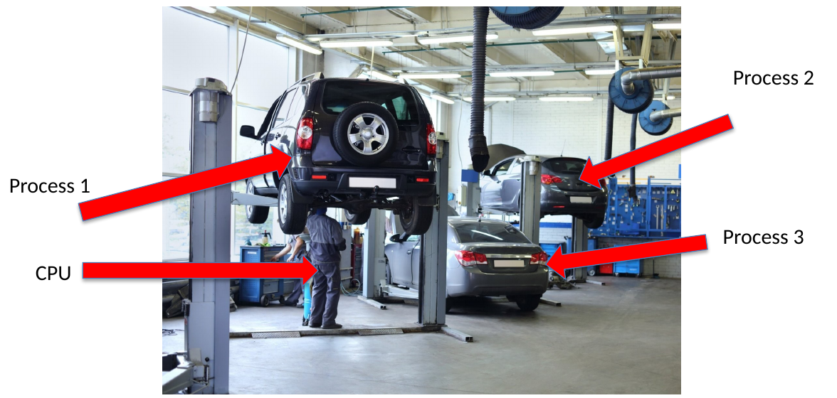
This is the central idea behind multiprogramming. Admitting several jobs creates opportunities to use a processor when another job cannot proceed. It does not make the missing part arrive sooner and does not let a single mechanic perform two independent operations simultaneously. Likewise, a single CPU can interleave execution and overlap it with device activity without executing two software instruction streams at the same instant in our simple model.
Two mechanics change the available capacity. They may work on two cars in parallel, provided that both jobs are ready and the mechanics have the necessary tools. The additional worker does not remove dependencies. If both need the same lift or diagnostic instrument, resource contention can still limit progress.

A useful analogy has boundaries. A CPU context switch preserves an execution state that can later resume precisely. Moving a mechanic between physical jobs may involve constraints that have no direct CPU equivalent. Use the analogy to distinguish readiness, service and waiting, then state the operating-system mechanism explicitly.
2. Urgency, duration and readiness
Before defining algorithms, ask what the service desk should optimize. Serving cars in arrival order is easy to explain. Serving short jobs first can reduce the typical wait. Giving urgent work priority may protect an important service. These policies can choose different cars from the same queue, and none is meaningful without its objective.
The instructor’s priority photograph motivates the question of urgency. A priority represents an ordering chosen by a policy. It does not, by itself, establish a deadline, explain whether work can be interrupted safely or prove that urgent work will finish in time.

The tyre-change and engine-repair photographs contrast service durations. For CPU scheduling, the useful quantity is often the next CPU burst rather than the entire lifetime of the program. A browser can remain open for hours while repeatedly executing short bursts after input. A computation can have a long burst even if the program eventually exits quickly compared with the browser.


Now distinguish two kinds of waiting. A ready car has everything it needs except the mechanic’s attention. A blocked car needs an external event, such as a part delivery. In an OS, a ready thread can make progress when scheduled. A blocked thread must first have its dependency satisfied. Increasing its CPU priority cannot produce missing input.
The distinction changes how we diagnose slow progress. A long ready-queue delay suggests competition for execution resources. A long device wait suggests a different constraint. The same program can move between both states many times, so calling the entire application “slow” does not identify a remedy.

3. CPU bursts, selection and dispatch
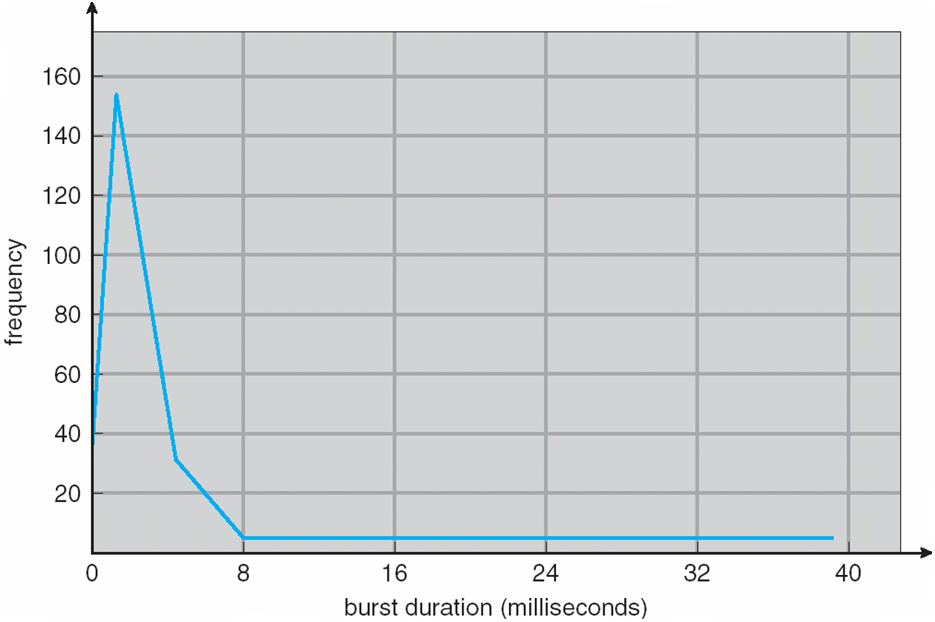
A CPU burst is an interval of processor work before the task blocks or otherwise leaves execution. Many workloads alternate computation with I/O waits. When one task blocks, the scheduler can select another ready task. This lets CPU and device activity overlap. The maximum benefit depends on the workload, because a collection of jobs that all wait for the same busy device may offer little ready work.
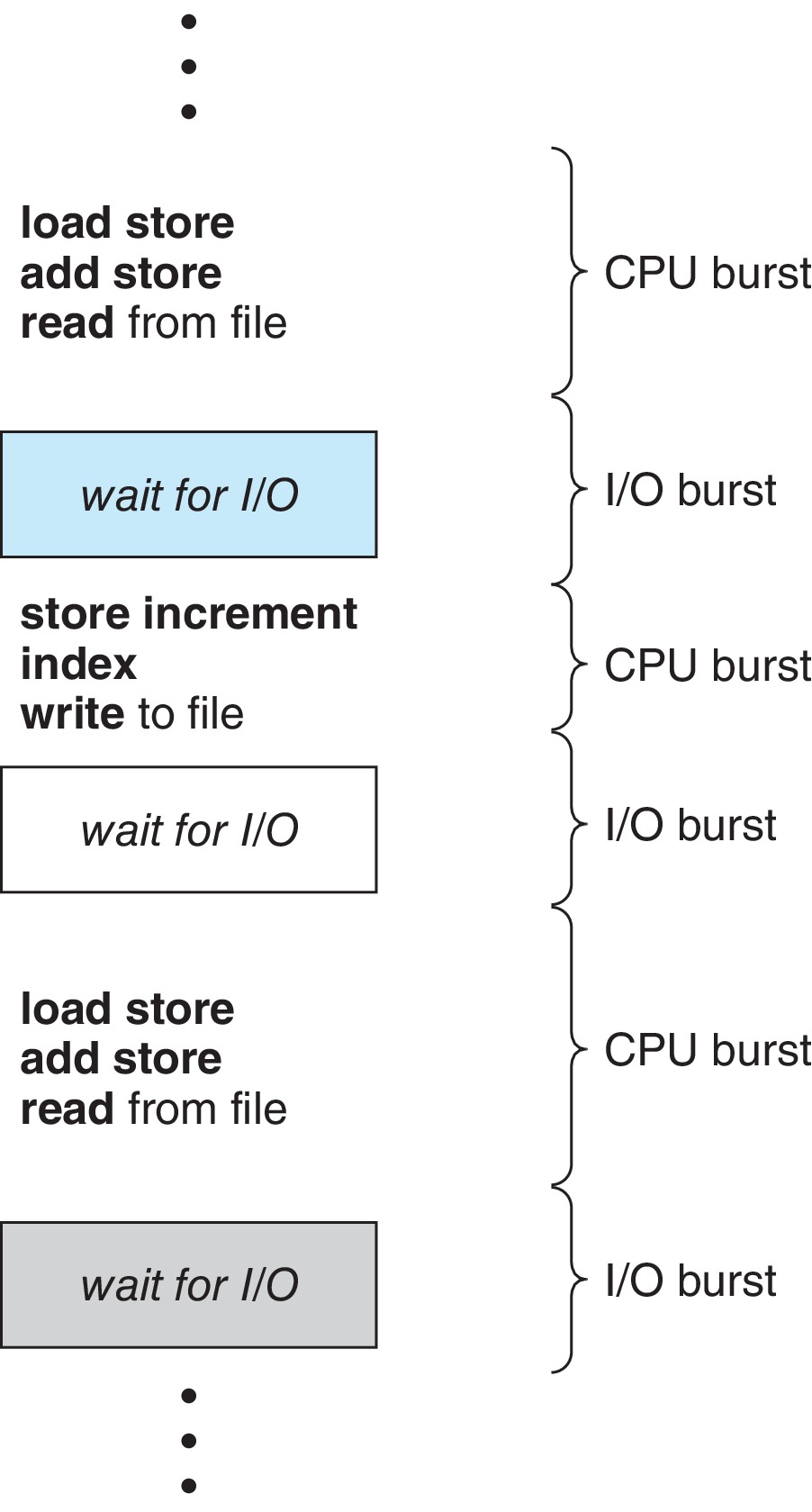
The burst histogram in the original materials illustrates a common teaching pattern: many short bursts and fewer long ones. Treat it as a workload illustration, not a measured distribution from our machines. Different applications and inputs can produce different distributions. A scheduling policy that benefits one mixture may perform poorly for another.
The scheduler chooses the eligible task. The dispatcher carries out the transfer so that task actually runs. The service desk illustrates the choice, while assigning the chosen job to a mechanic illustrates the transfer. Keeping the two concepts separate helps us distinguish policy from mechanism.


Dispatching can require saving registers, restoring another context and changing the execution environment. It consumes time even though it does not directly advance the application’s requested calculation. Cache and translation effects can add indirect costs. Our first timelines set these costs to zero so that policy decisions remain easy to see. That assumption must be restored when interpreting real performance.
Nonpreemptive scheduling lets a running burst continue until it finishes or blocks. Preemptive scheduling can return a still-runnable task to the ready queue. A timer interrupt or a wake-up may trigger reconsideration, but an interrupt does not prove that a different task ran. The scheduler may keep the current task. Preemption also creates more opportunities for shared-state interleavings, which motivates the next lecture on synchronization.
4. What does a good schedule mean?
CPU utilization measures the fraction of elapsed time for which the CPU is busy. Throughput counts completed work per unit time. These describe resource use and output, but they do not tell us whether an individual request responds promptly. A system can keep its CPU fully occupied while a short interactive request waits behind a long calculation.
For each job, distinguish arrival A, first start S, completion C and total CPU demand B. Turnaround T = C − A measures the full lifetime after arrival. Response R = S − A measures the delay until first CPU service in our scheduling exercises. An application-level response may require more work before anything becomes visible to a user. Waiting W counts time spent ready but not executing.
For a job with one CPU-only burst and no other delays, W = C − A − B. With I/O, turnaround also includes blocked time. Subtracting only CPU time would incorrectly classify device waiting as ready-queue waiting. Always match the accounting formula to the workload model.
| Quantity | Given or calculated value |
|---|---|
| Arrival A | 2 |
| First start S | 5 |
| Completion C | 12 |
| CPU demand B | 4 |
| Turnaround T | 12 − 2 = 10 |
| Waiting W | 10 − 4 = 6 |
| Response R | 5 − 2 = 3 |
The job first waits three units before it receives CPU service. It later accumulates another three units of ready waiting. Its response time therefore differs from its total waiting time. This is why measuring the first start alone cannot tell us how often a job was delayed later.
Use averages carefully. A small mean waiting time can hide one very long wait. Fairness asks how service is distributed, and real-time requirements ask whether particular deadlines hold. A policy comparison should state which of these objectives matters before claiming that one schedule is better.
5. FCFS and the convoy effect
First-come, first-served scheduling runs jobs in ready-queue arrival order. In our first workload, P1 needs 24 CPU units, P2 needs 3 and P3 needs 3. All arrive at time 0. We explicitly break that simultaneous-arrival tie using the order P1, P2, P3. There is one processor, no I/O and no switching overhead.
P1 occupies [0,24), P2 occupies [24,27), and P3 occupies [27,30). The half-open interval convention means that P1 finishes at 24 and P2 may begin at that same boundary. Read the labels and boundary values separately: the widths show duration, while the boundary numbers give the exact event times.

| Job | A | B | S | C | W | R | T |
|---|---|---|---|---|---|---|---|
| P1 | 0 | 24 | 0 | 24 | 0 | 0 | 24 |
| P2 | 0 | 3 | 24 | 27 | 24 | 24 | 27 |
| P3 | 0 | 3 | 27 | 30 | 27 | 27 | 30 |
The mean waiting time is (0 + 24 + 27)/3 = 17. Mean turnaround is (24 + 27 + 30)/3 = 27. Since this is nonpreemptive work with all arrivals at zero, each job’s first delay is also its whole waiting time.
Now change only the initial tie order to P2, P3, P1. The schedule becomes [0,3), [3,6), [6,30). Waiting times in P1/P2/P3 order are 6, 0 and 3, so the mean is 3. Mean turnaround falls to (30 + 3 + 6)/3 = 13. Total CPU demand and the final completion time remain 30.

The contrast shows how arrival order can dominate the experience of short jobs. The convoy effect extends this reasoning to alternating CPU and I/O work. Short tasks behind a long CPU burst cannot issue their next device requests until they run. When they eventually move to I/O, the CPU may have fewer useful alternatives. A single-burst chart illustrates the queueing delay, while the full convoy explanation also considers device activity.
For practice, change P1’s demand from 24 to 12 while keeping the other assumptions. Predict whether throughput, mean waiting and first response change in the same proportion. They do not: different metrics combine the event times differently.
6. Shortest job first and uncertain bursts
Nonpreemptive shortest job first selects the smallest next burst among ready work. For a fixed collection available together, with known burst lengths and zero overhead, it minimizes average waiting. The qualification matters. A real scheduler normally does not know future CPU demand exactly, and jobs can arrive after a decision has begun.
The exchange argument explains the result. Suppose adjacent ready jobs have lengths x and y, with x ≤ y. Running x first makes the second job wait x. Running y first makes the second wait y. Both orders finish the pair at the same time, leaving later jobs unaffected. Putting the shorter job first cannot increase the total wait. Repeatedly exchanging inverted pairs yields ascending burst order.
For P1/P2/P3/P4 bursts 6/8/7/3 with arrivals all zero, the order is P4, P1, P3, P2. Completion boundaries are 3, 9, 16 and 24. Waiting times in process-number order are 3, 16, 9 and 0, with mean 7.

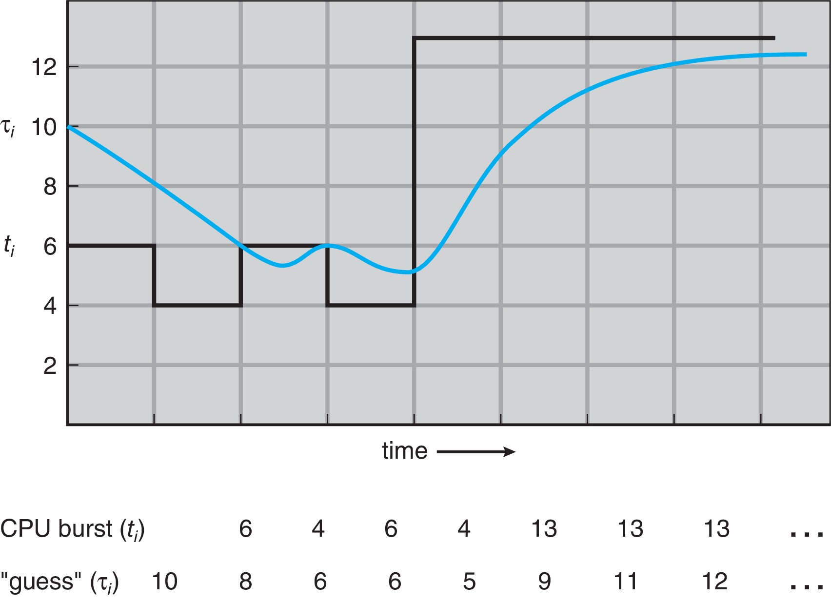
One approach to unknown bursts is exponential averaging. Let τ be the previous estimate, t the observed burst and α a weight from zero to one. The next estimate is αt + (1 − α)τ. With α = 0.5 and τ = 10, observing 6 produces an estimate of 8. Observing 4 next produces 6. The estimate incorporates history without retaining every old observation separately.
A large α responds strongly to recent behaviour. A small α smooths short fluctuations but takes longer to follow a sustained change. At α = 0, observations never update the estimate. At α = 1, only the latest observation matters. These are predictions of typical future demand, not safe worst-case bounds for a hard real-time guarantee.
Could a long ready job wait forever under SJF?
Yes, if shorter work keeps arriving and always wins at each selection opportunity. Minimizing a mean for one fixed batch does not establish starvation freedom for an ongoing workload.
7. Shortest remaining time first
SRTF adds preemption to duration-based selection. Whenever arrivals or completions change the ready set, compare remaining demands. Comparing original burst lengths would be wrong after a job has already consumed service. We keep the current job on an exact tie, so the tie rule is reproducible.
| Job | Arrival | Burst |
|---|---|---|
| P1 | 0 | 8 |
| P2 | 1 | 4 |
| P3 | 2 | 9 |
| P4 | 3 | 5 |
P1 begins at 0. At time 1 it has seven units left, while newly arrived P2 needs four, so P2 preempts it. At time 2, P2 has three left and P3 needs nine. At time 3, P2 has two left and P4 needs five. P2 therefore continues to completion at 5.
At 5, compare P1’s seven remaining units, P3’s nine and P4’s five. P4 runs until 10. P1 then resumes until 17, and P3 runs until 26. P1’s original burst has been split into two intervals, [0,1) and [10,17).

| Job | Completion | Turnaround | Waiting | Response |
|---|---|---|---|---|
| P1 | 17 | 17 | 9 | 0 |
| P2 | 5 | 4 | 0 | 0 |
| P3 | 26 | 24 | 15 | 15 |
| P4 | 10 | 7 | 2 | 2 |
Mean waiting is (9 + 0 + 15 + 2)/4 = 6.5. Mean response is (0 + 0 + 15 + 2)/4 = 4.25. P1 demonstrates the difference clearly: it receives immediate first service but waits for nine units after preemption.
A reliable calculation first constructs a legal schedule, then extracts first starts and completions, and only then computes metrics. Do not infer waiting directly from a bar’s horizontal position when the same job appears in several bars. Check that each job’s total executed duration equals its demand and that no interval runs a job before arrival.
8. Round robin and quantum cost
Round robin gives each runnable job at most a quantum q before returning unfinished work to the queue tail. A job can finish or block earlier. This shares access without predicting burst lengths. Queue order still matters, especially for first response, and a complete specification must say how arrivals at a quantum boundary are ordered.
For the original 24/3/3 workload, all jobs arrive at zero and q = 4. P1 runs from 0 to 4, P2 from 4 to 7, and P3 from 7 to 10. P1 then uses the remaining 20 units and completes at 30. The textbook chart marks subsequent quantum boundaries even though only P1 remains. Those boundaries do not necessarily correspond to switches to another task.

| Job | Completion | Waiting | First response |
|---|---|---|---|
| P1 | 30 | 6 | 0 |
| P2 | 7 | 4 | 4 |
| P3 | 10 | 7 | 7 |
Mean waiting is 17/3, approximately 5.67. Mean response is 11/3, approximately 3.67. For this particular workload, SJF’s mean is even smaller, yet round robin gives P1 earlier first service than SJF. The policy choice should follow the desired service distribution rather than a slogan that one algorithm is always more responsive.
With n continuously runnable equal-priority peers, no new arrivals and zero overhead, the gap between a task’s turns is at most (n − 1)q. Higher-priority interference, additional tasks and switching costs invalidate that simple bound. State the model before using the formula.
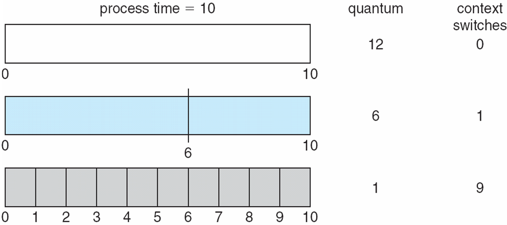
To expose overhead, imagine saturated work alternating between tasks. A useful quantum of q followed by switch cost s gives an approximate useful fraction q/(q+s). For q = 4 ms and s = 0.2 ms, this is 4/4.2 ≈ 95.24%. With q = 1 ms and the same s, it becomes 1/1.2 ≈ 83.33%. These are assumed costs for a simple model, not measurements of Ubuntu.
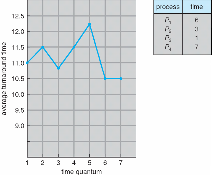
Turnaround need not improve monotonically as q changes. Different jobs finish at different boundaries, changing later queue positions. Large quanta approach FCFS; extremely short ones can waste time switching. The original graph is useful precisely because its shape discourages a universal rule based on quantum alone.
9. Priorities, starvation and feedback
A priority policy orders eligible tasks by importance as defined by the system. Priorities can be fixed or dynamic, and the policy can be preemptive or nonpreemptive. Numerical conventions vary. The following textbook example treats smaller numbers as higher priority, so the convention is part of the input rather than something to guess.
| Job | Burst | Priority |
|---|---|---|
| P1 | 10 | 3 |
| P2 | 1 | 1 |
| P3 | 2 | 4 |
| P4 | 1 | 5 |
| P5 | 5 | 2 |
The order is P2, P5, P1, P3, P4. Starts are 0, 1, 6, 16 and 18 in that execution order. Waiting in P1…P5 order is 6, 0, 16, 18, 1. The mean is 41/5 = 8.2. Switching the numerical convention would produce a different schedule, so explicitly write “smaller is higher” beside the input.

Starvation occurs when an eligible task is postponed indefinitely while others keep receiving service. Round robin among equal-priority peers does not protect a low-priority task from an endless stream of higher-priority work. Aging raises the effective priority of waiting tasks, but the precise progress guarantee depends on how fast priorities change, how ties work and what higher-priority load is admitted.
Multilevel queues separate classes of work and define selection within and between those classes. If the top queue always wins, lower queues may starve. A multilevel feedback queue additionally allows movement between levels based on observed behaviour. It uses recent service history as evidence rather than asking for an exact future burst.
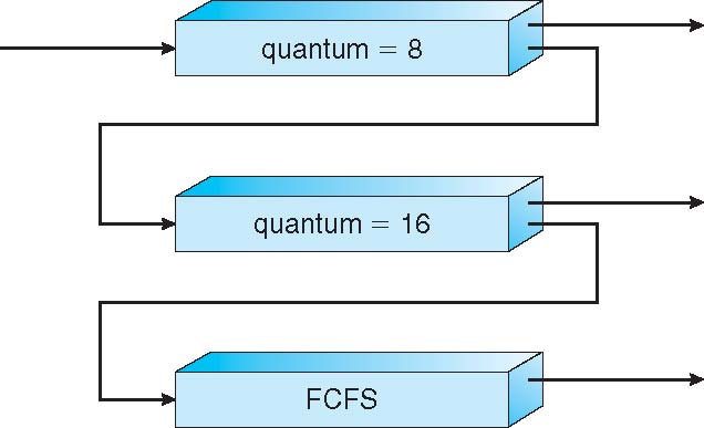
In the illustrated policy, a new task starts in Q0. Consuming all eight units without completion demotes it to Q1. Consuming sixteen more moves it to Q2. A solitary 30-unit CPU job therefore receives 8 + 16 + 6 units and finishes at 30 when overhead is zero. Competition from higher queues can add delays, but queue changes do not alter the useful demand.
This picture is an outline rather than a complete algorithm. We must also define how an I/O return affects priority, whether a task can preserve a level by yielding early, and when long-waiting tasks receive boosts. Accounting for a total allotment across several short runs helps prevent a task from gaming a per-run demotion rule. Periodic boosts can restore opportunities for low-level work.
10. Multiple execution resources and locality
With multiple CPUs, scheduling decides both when and where a thread runs. A common ready queue simplifies the conceptual choice: each free CPU selects available work. However, many CPUs accessing one structure can create contention. Per-CPU queues reduce this shared access and help keep work near familiar cache contents, but they can become unevenly loaded.
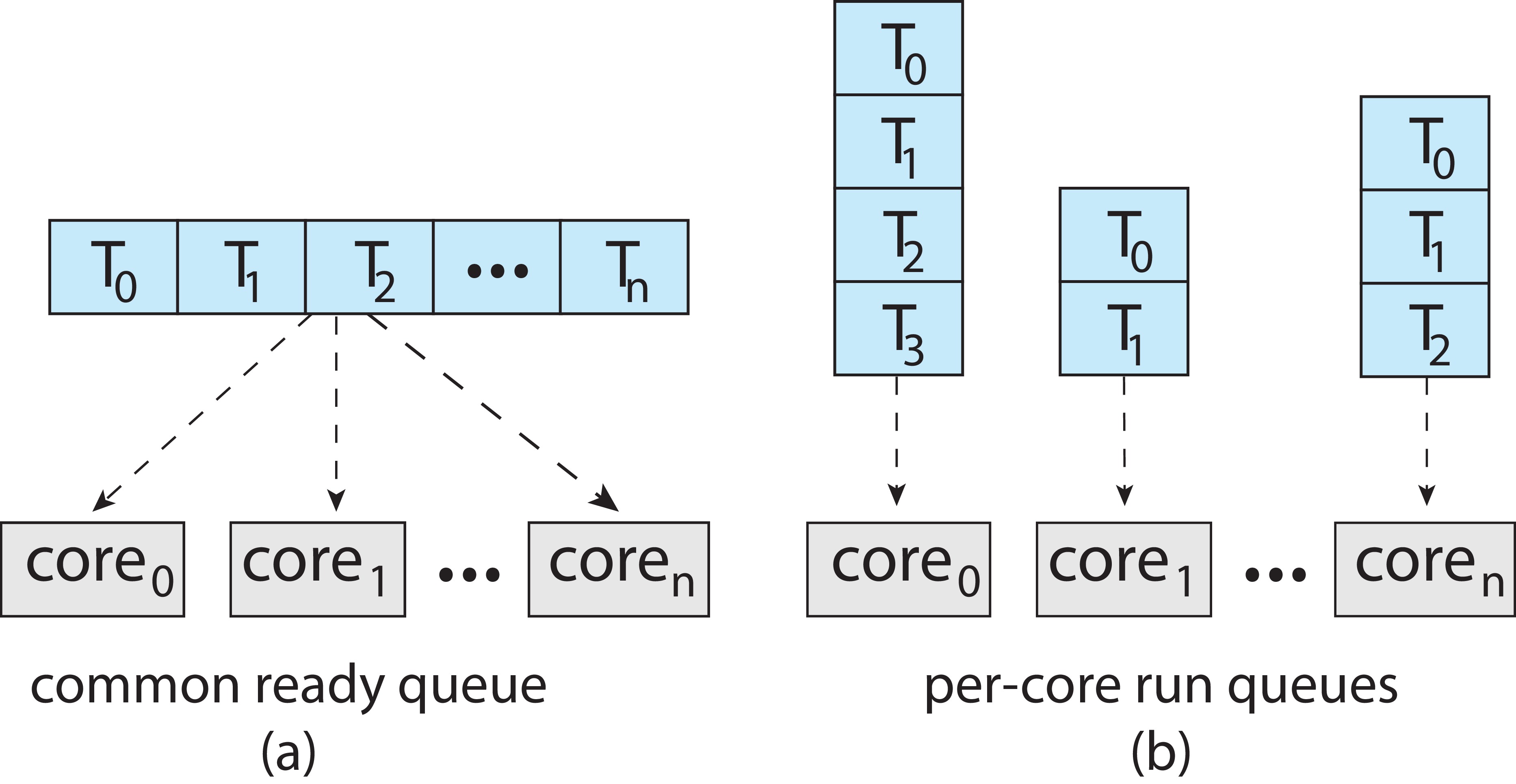
Load balancing moves runnable work so that an idle execution resource can help a busy one. Affinity pulls in the opposite direction when migration discards useful locality. A task that repeatedly touches the same working set may benefit from the CPU where its data are cached. On a NUMA machine, the placement of memory relative to CPUs adds another cost.
Logical CPU identifiers do not directly count independent physical cores. Hardware threads within a core share execution resources. The original compute/stall illustration shows why overlapping activity can improve use of those resources, but it does not establish a twofold speedup. The result depends on which resources the threads compete for.
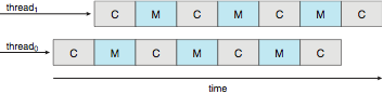
A runtime can also schedule user-level work inside its assigned kernel threads. The kernel does not automatically see every user-level task as a separate runnable entity. When a VM hosts the workload, the guest’s choices additionally depend on when the host schedules its virtual CPUs. A clean classroom timeline describes the chosen model, while measurements must record these additional scheduling layers.
An affinity mask constrains where work may run. It is not a CPU reservation and does not exclude other tasks or interrupts. Use affinity in a controlled observation to make contention easier to interpret, then keep that limitation visible in the explanation.
11. Real-time requirements and the task model
Real-time correctness depends on when results arrive. A hard requirement makes deadline satisfaction part of correctness under specified conditions. A soft requirement tolerates some lateness with reduced service quality. The distinction concerns consequences and requirements, not whether a processor is fast or whether the average response looks small.
A task can generate a sequence of jobs. A job is one released instance with release time r, required execution C and absolute deadline d. A periodic task releases a new job every T time units. A relative deadline D gives d = r + D. Distinguishing task from job prevents us from comparing the next period of one task with the deadline of the wrong job.
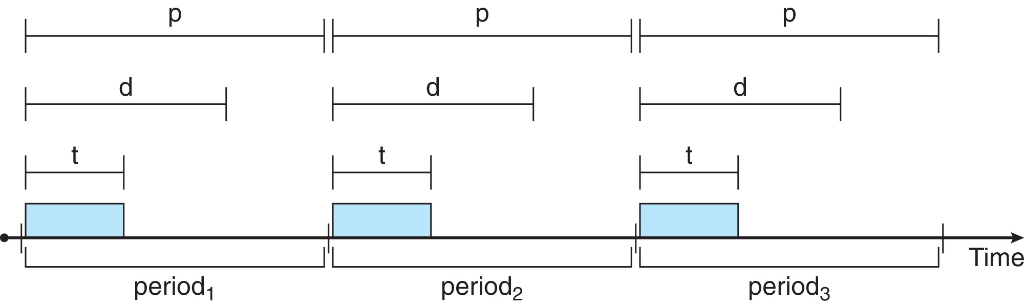
For the introductory RM and EDF calculations, assume one processor, independent periodic tasks, simultaneous first releases, full preemption and zero scheduling cost. Set D = T. Treat C as a valid worst-case execution bound, not a sample average. There is no resource blocking or release jitter. These assumptions make the feasibility statements precise.
Utilization U = Σ(Ci/Ti) describes aggregate required service. It is an average demand fraction over the repeating workload. A low fraction alone does not establish that all deadlines can be met by every priority rule. Demand can compete within specific windows, and the selected algorithm determines which job waits.
Before useful execution begins, an event may incur interrupt delay, handler work and dispatch latency. A ready high-priority task may also depend on a resource held by lower-priority work. A full real-time design needs bounds for these sources of delay. Our zero-cost model is a starting point for reasoning, not evidence of an actual machine’s worst-case timing.
12. Rate-monotonic scheduling
RM gives the shorter-period task the higher fixed priority. New jobs of that task can preempt lower-priority work. The priority ordering does not change from job to job. In Example A, P1 has C1 = 20 and T1 = 50, while P2 has C2 = 35 and T2 = 100. All numbers in this and the following real-time examples are milliseconds.
At zero, P1 runs first and finishes at 20. P2 executes 30 of its 35 units between 20 and 50. A new P1 job arrives at 50 and preempts it, running until 70. P2 then finishes its remaining five units at 75, before its deadline at 100. Both jobs have met their deadlines.

The utilization is 20/50 + 35/100 = 0.75. Under the stated model, a sufficient RM schedulability condition for n tasks is U ≤ n(21/n − 1). For two tasks the bound is approximately 0.8284, so Example A passes. “Sufficient” is essential: failing this bound means the test has not established feasibility. It does not establish a deadline miss.
For a counterexample to the mistaken interpretation, consider tasks (C,T) = (1,2) and (2,4), with D = T. RM runs the first task from 0 to 1, the second from 1 to 2, the first from 2 to 3, then the second from 3 to 4. The pattern repeats. Utilization is 1, above the general two-task bound, yet every deadline is met.
Example B changes the workload to P1 = (25,50) and P2 = (35,80). Utilization is 0.5 + 0.4375 = 0.9375. P1 still has higher RM priority. It runs 0–25, P2 runs 25–50, and the next P1 job runs 50–75. P2 still needs ten units at 75 but its deadline is 80. It finishes at 85, five units late.

The same interference can be expressed through response-time iteration for the lower-priority task. Here R denotes release-to-completion time, unlike the first-service response metric used earlier. Begin with R0 = C2 = 35 and apply R(next) = 35 + ceil(R/50) × 25. The values become 60, then 85, then remain 85. Each ceiling counts higher-priority jobs that can interfere during the response interval. The fixed point exceeds D2 = 80, agreeing with the timeline. This recurrence uses our no-blocking, fully preemptible task model.
13. EDF and absolute deadlines
EDF assigns the highest current priority to the ready job with the earliest absolute deadline. Unlike RM, that ordering can change between jobs of the same two tasks. At time 50 in Example B, the unfinished P2 job still has deadline 80. The new P1 job has deadline 100. EDF therefore continues P2, allowing it to finish at 60. P1 then runs until 85, also meeting its deadline.
At time 80, a second P2 job is released with deadline 160. It waits until P1 finishes at 85, runs until 100, then is preempted by P1’s new job with deadline 150. P1 completes at 125. P2 resumes and completes at 145. There is an idle interval until 150. At each event, compare the deadlines of released, unfinished jobs rather than task periods alone.

| Interval | Executing job | Absolute deadline |
|---|---|---|
| 0–25 | P1 released 0 | 50 |
| 25–60 | P2 released 0 | 80 |
| 60–85 | P1 released 50 | 100 |
| 85–100 | P2 released 80 | 160 |
| 100–125 | P1 released 100 | 150 |
| 125–145 | P2 released 80 | 160 |
| 145–150 | Idle | — |
| 150–175 | P1 released 150 | 200 |
| 175–210 | P2 released 160 | 240 |
| 210–235 | P1 released 200 | 250 |
Under our independent, fully preemptible single-processor model with D = T, U ≤ 1 is the exact EDF utilization condition. Example B’s U = 0.9375 therefore supports feasibility even though RM fails. A trace explains individual choices; the theorem supplies the wider guarantee under the assumptions.
When deadlines are shorter than periods, utilization alone no longer captures the tightest demand windows. With blocking, switching costs, release jitter or several processors, further analysis is necessary. Do not take a classroom feasibility result and apply it to an arbitrary deployed system without checking every assumption.
Priority inversion illustrates one omitted dependency. If high-priority H needs a lock held by low-priority L, medium-priority M can preempt L and indirectly delay H. Priority inheritance can temporarily increase the lock owner’s priority, but valid timing bounds still depend on the locking protocol and critical-section lengths. Synchronization is therefore part of real-time reasoning, not merely a separate correctness topic.
14. Linux context and optional Ubuntu observation
The older deck explains CFS using virtual runtime. Current kernel documentation describes a transition toward EEVDF beginning with Linux 6.6. EEVDF’s virtual deadlines guide fair service among eligible tasks. They do not promise an application will finish by a wall-clock deadline. Check the installed kernel before interpreting observations. See the kernel’s EEVDF documentation.
SCHED_DEADLINE is a separate policy combining EDF with reservation mechanisms. Ordinary nice values influence relative service rather than hard deadlines. Linux SCHED_FIFO and SCHED_RR use real-time priorities, with RR sharing service among peers. The scheduling manual describes these interfaces. The activity below uses ordinary policies.
This is optional study practice, not a released graded assignment. AI assistance is permitted. Use it to propose explanations or check your arithmetic, then compare those explanations with code, documentation and recorded observations. Keep the raw output so you can distinguish what happened from what you expected. The program was compiled and run on the preparation host, macOS. The Ubuntu-specific commands remain to be tested on the selected course environment.
uname -r
lscpu
ps -o pid,cls,ni,psr,comm -p "$$"
chrt -p "$$"
taskset -pc "$$"
Record the environment, the allowed CPU list and the scheduling policy. A sampled CPU number is not evidence of continuous execution there. Affinity restricts placement but does not provide exclusive use. These read-only commands inspect the current shell. Consult taskset(1), chrt(1) and ps(1) for installed-tool details.
The following program stops after about 0.75 seconds of consumed process CPU time. It also measures elapsed time. Because it checks the clock after a batch of arithmetic, the CPU total can slightly exceed the target. Under contention it may take longer in elapsed time to acquire the same CPU service. The unsigned arithmetic has defined wraparound, and the volatile variable keeps the work observable to the compiler.
#define _POSIX_C_SOURCE 200809L
#include <stdint.h>
#include <stdio.h>
#include <stdlib.h>
#include <time.h>

static double seconds(clockid_t id) {
    struct timespec ts;
    if (clock_gettime(id, &ts) != 0) { perror("clock_gettime"); exit(1); }
    return (double)ts.tv_sec + (double)ts.tv_nsec / 1e9;
}
int main(void) {
    const double demand = 0.75; /* CPU seconds, not elapsed seconds. */
    const double wall0 = seconds(CLOCK_MONOTONIC);
    const double cpu0 = seconds(CLOCK_PROCESS_CPUTIME_ID);
    volatile uint64_t state = 1;
    unsigned long batches = 0;
    do {
        for (int i = 0; i < 100000; ++i)
            state = state * UINT64_C(6364136223846793005) + 1;
        ++batches;
    } while (seconds(CLOCK_PROCESS_CPUTIME_ID) - cpu0 < demand);
    const double cpu = seconds(CLOCK_PROCESS_CPUTIME_ID) - cpu0;
    const double elapsed = seconds(CLOCK_MONOTONIC) - wall0;
    printf("cpu_s=%.6f elapsed_s=%.6f batches=%lu checksum=%llu\n",
           cpu, elapsed, batches, (unsigned long long)state);
    return 0;
}
Download cpu-work.c. Compile with a C compiler using cc -O2 -std=c11 -Wall -Wextra cpu-work.c -o cpu-work. Run ./cpu-work once before changing the experiment. The output includes CPU seconds, elapsed seconds and an arithmetic-batch count.
To create a comparison, choose one allowed logical CPU from the earlier affinity output. Replace the value below with that CPU number. Start two ordinary workers on that same CPU, with nice values 0 and 10. No administrator privilege is required for this reduction in the second worker’s priority. Do not assume CPU 0 is available inside every container or virtual environment.
cpu_id=2  # Replace 2 with one CPU allowed by taskset -pc "$$".
taskset -c "$cpu_id" ./cpu-work > normal.txt &
worker_normal=$!
taskset -c "$cpu_id" nice -n 10 ./cpu-work > nice10.txt &
worker_nice=$!
wait "$worker_normal"
wait "$worker_nice"
cat normal.txt nice10.txt
Predict which worker is likely to accumulate its CPU demand first. Repeat the experiment, reverse the launch order, and compare with two equal-nice workers. Retain the elapsed times, CPU times and environment notes. Launching background jobs does not release them at an exactly simultaneous instant, and the program that finishes first changes the competition faced by the survivor.
This experiment can reveal contention and relative service. It cannot prove an exact CPU-share ratio, identify the scheduler solely from timing, or establish a hard real-time bound. Background load, virtual CPU allocation, affinity, compiler behaviour and power management can affect the observations. Explain differences using evidence rather than forcing them to match the ideal classroom schedules.
15. Evaluation and study questions
Deterministic schedules make assumptions explicit and permit exact checks. Simulation explores many arrival sequences and demands, but it only models the mechanisms that were included. Measurement incorporates actual system costs and interference, while making reproducibility harder. These forms of evidence answer different questions. Use the same workload and metric when comparing policies, and report the distribution of delays when a mean conceals important variation.
Little’s law offers an additional consistency check for a stable queue: Lq = λWq. If the average queue contains fourteen waiting jobs and seven jobs enter per second, average queue wait is two seconds. The boundaries must match. If the count includes the running job, use time in the system rather than queue-only waiting. A perpetually growing overloaded queue does not supply the stable averages assumed by this calculation.
1. A task has response time zero. Must its waiting time also be zero?
No. It can begin immediately, then spend time ready after preemption. P1 in the SRTF example responds at zero and accumulates nine units of waiting.
2. Why do the two FCFS orders finish at the same time?
Both perform the same thirty units of useful CPU work with no idle intervals or overhead. Their individual completion times differ, changing the averages.
3. What happens to RR when the quantum exceeds every burst?
For the all-ready single-burst workload, jobs finish on their first turn, so the order and timing match FCFS. With arrivals, blocking or other policy layers, restate the conditions before making the comparison.
4. Can low utilization establish every RM deadline?
No general claim follows merely from U being below one. Example B uses 0.9375 and misses under RM. The sufficient RM bound is stronger, and a failed bound requires further analysis.
5. Does exceeding the RM bound establish failure?
No. The harmonic example (1,2), (2,4) has utilization one and meets its deadlines. Distinguish a sufficient test from a necessary condition.
6. At time 50 in Example B, why do RM and EDF disagree?
RM favours P1 because its period is shorter. EDF favours the unfinished P2 job because its deadline of eighty is earlier than the new P1 job’s deadline of one hundred.
7. What does pinning both workers accomplish?
It restricts both to the chosen allowed logical CPU, making them compete there. It does not isolate that CPU from unrelated work or guarantee simultaneous starts.
8. Can an observed maximum execution time serve as a guaranteed WCET?
An observed maximum is evidence about the runs performed. A guaranteed worst-case bound needs a justification covering the relevant inputs and operating conditions, including interference and platform behaviour.
9. What must a scheduling simulator check?
No execution before release, no negative remaining demand, no overlapping execution on one modeled CPU, conservation of each job’s demand, consistent tie rules and correct deadlines. Calculate metrics from events rather than guessed chart positions.
10. How should AI assistance be used for a timeline?
Ask for the assumptions and event sequence, then independently verify arrivals, remaining demands, first starts and completion times. A fluent explanation can contain an illegal preemption or an arithmetic error.
For a complete study pass, reproduce FCFS, SRTF and RR without looking at the answers. Then trace Example B under both RM and EDF through time 160. Explain every change in the executing job and every idle interval. Finally, write one paragraph about which assumptions the Ubuntu experiment satisfies and which it does not. This connects the mathematical model to evidence without treating either as a substitute for the other.
16. References and further study
The main reference is Abraham Silberschatz, Peter B. Galvin and Greg Gagne, Operating System Concepts, 10th edition (Wiley, 2018), Chapter 5. Use §§5.1–5.3 for bursts, criteria and algorithms, §5.4 for thread scheduling, §5.5 for multiprocessor considerations, §5.6 for real-time principles, and §5.8 for evaluation. In particular, §§5.6.3–5.6.4 develop the RM and EDF examples retained here. Section numbers refer to the supplied edition.
Figures credited to OSC come from the authors’ official 10th-edition slides. Other retained figures come from Mehmet Göktürk’s instructor scheduling deck and preserve its teaching sequence. The chapter explanations, full accounting tables and practice program are adaptations written for CSE513. Historical diagrams are conceptual illustrations rather than current measurements.
For complementary explanations, consult Remzi H. Arpaci-Dusseau and Andrea C. Arpaci-Dusseau’s Operating Systems: Three Easy Pieces: Scheduling: Introduction, The Multi-Level Feedback Queue, and the authors’ chapter index. These links provide further reading without redistributing the books.
The Linux references linked in Section 14 were checked during preparation on 29 September 2026. Local manual pages and the installed kernel determine the environment used for actual practice. Required viewing has not been assigned for Week 2.