CSE 101 · WEEK 12 · READING
Artificial intelligence and data structures
From rules and search to learning systems; from records to connected nodes.
Read the AI concepts first, then trace the node-and-link examples. Try each Check before opening its answer. The detailed reference galleries are optional. Lab 11 focuses on supplied singly linked lists on the PC; tree and graph implementation is not required. Click any figure to enlarge it. Wide code and tables scroll sideways.
1. Intelligence is a question about tasks and evidence

A robot moving through a room needs more than a motor command. It must obtain observations, represent what matters, choose an action and assess what happened. Shakey, developed at SRI from 1966 to 1972, is a historical example linking perception, planning and physical action. Its photograph is a reminder that artificial intelligence includes interaction with the world, not only conversation. See SRI’s Shakey history.
Artificial intelligence is a broad area concerned with systems performing tasks associated with intelligent behavior. Machine learning is one family of methods within it: models are fitted from data or experience. Deep learning is a family of machine learning using multilayer neural networks. These terms are related, but not interchangeable. A planner using explicit rules and search can be an AI system without learning its rules from examples.
Turing’s imitation game examined behavior through conversation. Success on one behavioral test does not establish general competence or settle questions about consciousness. For engineering, begin with a concrete task: what inputs does the system receive, what output is useful, and what evidence would show that it works? A chess result, an image classification score and a robot’s navigation reliability measure different achievements.
Check: Must every AI system train a neural network?
No. Explicit rules, symbolic representations and search can support intelligent behavior. Learning can also be combined with these methods.
2. Rules need representations and reliable premises
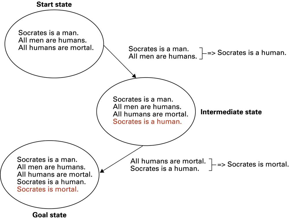
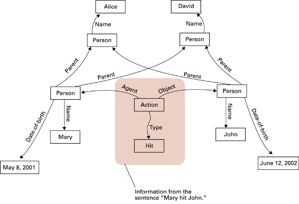
An expert system separates knowledge from the procedure that applies it. Facts describe a situation; rules connect conditions to conclusions. In a simplified equipment example, observing a commanded motor with zero current might lead to a recommendation to inspect the circuit. This is a teaching illustration, not a real diagnostic or safety procedure: missing facts can change the conclusion.
Deduction follows implications from premises. If a rule says that every item of class A has property B, and a particular item is known to be A, B follows under that rule. The inference can be valid even when a premise is factually wrong. The quality of the knowledge base therefore matters as much as the inference mechanism.
A semantic network represents concepts and named relationships. A link can mean “is a kind of,” “has a part” or another explicit relation. Do not interpret all arrows as the same operation. These symbolic links differ from weighted connections in a neural network: a neural weight is a numerical parameter, not automatically a human-readable proposition.
Check: If a rule system can explain which rule it used, does that prove its answer is correct?
No. The explanation exposes the reasoning path. The facts and rules still need to be appropriate and correct.
3. Represent a problem before searching for a solution
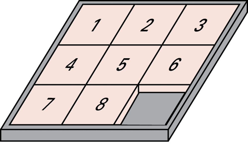
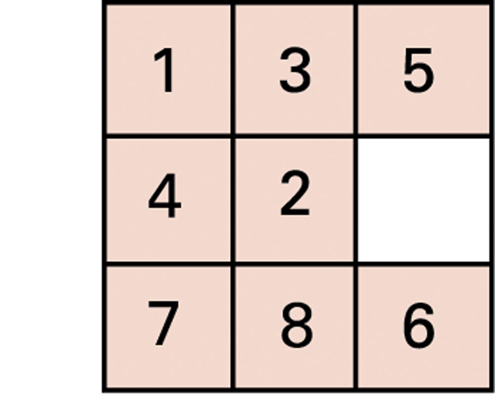
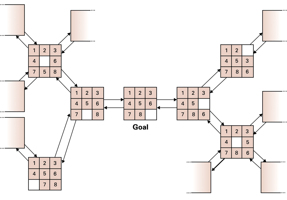
The sliding-tile puzzle makes a search problem visible. A state records the tile arrangement. An action moves a neighboring tile into the empty position. A goal test compares the state with the required arrangement. A solution is a legal sequence of actions, not merely a picture of the desired result. This separation also applies to route planning and game playing.
A state graph describes possible states and transitions. A search tree records exploration paths. Different paths can reach the same state, so the tree may repeat a state that appears once in the graph. Repeated-state handling prevents wasted exploration and, in some procedures, helps avoid cycling forever.
Week 8 introduced the cost of examining alternatives. Here the question is how domain knowledge can guide which alternatives to explore. A program still needs an exact representation, legal transitions and a correct goal test. Calling it AI does not remove those algorithmic responsibilities.
Check: If two move sequences reach the same board arrangement, must they be different states?
No. They are different paths to the same state, assuming the board arrangement contains all information relevant to future moves.
4. A heuristic guides search without being an oracle
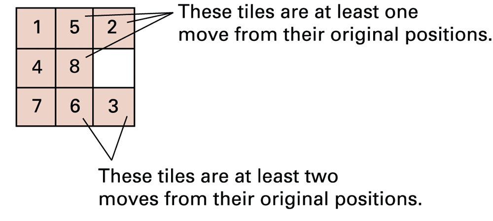
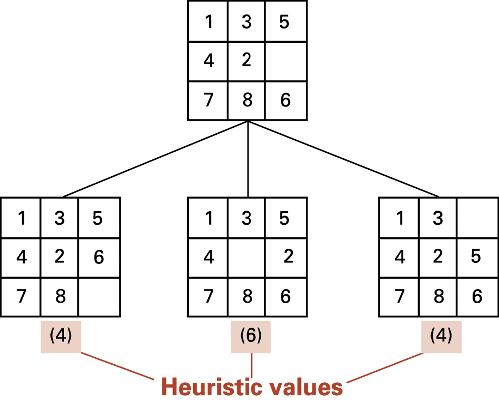
A heuristic h estimates the remaining effort. For the pictured puzzle, Manhattan distance counts horizontal and vertical displacement from each numbered tile’s target, ignoring the blank. The shown displaced tiles contribute 1 + 1 + 1 + 2 + 2 = 7. It is an estimate because legal moves may require temporary detours.
Greedy best-first search prioritizes a small h. A* instead combines the cost already paid, g, with the estimate remaining, h, using f = g + h. The original procedure shown later uses h alone and should not be called A*. A promising-looking state is not necessarily on the least-cost complete route.
Optimality claims require assumptions about costs, the heuristic and repeated-state handling. For the standard unit-cost sliding puzzle, the sum of numbered-tile Manhattan distances is a lower bound: a move changes one numbered tile’s distance by at most one. That does not turn every procedure using the estimate into an optimal search algorithm.
Check: Two candidates have (g,h) = (20,2) and (5,4). Which does greedy prefer, and which has smaller A* score?
Greedy prefers h = 2. Their g + h scores are 22 and 9, so A* prioritizes the second by that score. This comparison alone does not prove which complete route is optimal.
5. Search and learning can cooperate
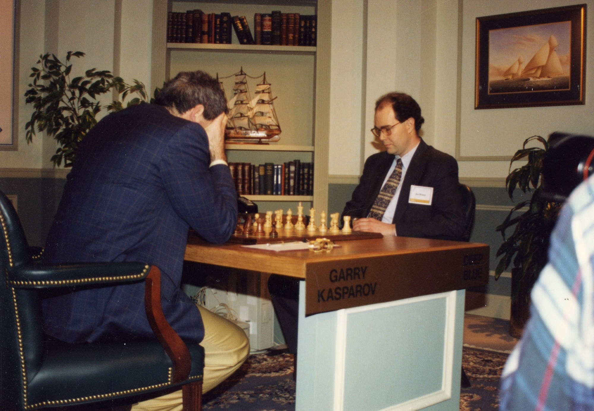

Deep Blue defeated Garry Kasparov in their 1997 match. Its success illustrates the power of extensive search, evaluation and specialized engineering in a well-defined game. AlphaGo combined learned policy and value information with search. Neither result means that one identical method solves every problem described as intelligent.
A game supplies legal moves and a clear result. Real deployments may instead have noisy observations, delayed feedback, changing conditions or disputed objectives. A system that is excellent within one environment can fail when those assumptions change. Identify the rules of the evaluation before transferring the conclusion to another task.
The photographs are credited to IBM and Google DeepMind. The point of the comparison is methodological: learned estimates can help choose useful branches, while explicit search organizes the alternatives.
Check: Does using a learned evaluation function mean a system no longer performs search?
No. Learning and search can serve different roles within the same system.
6. What changes when a model learns?
In supervised learning, an example contains input information and a target answer. A model makes a prediction; a loss measures its discrepancy from the target; training adjusts parameters to improve the objective. Features are the representation supplied to the model. Parameters are quantities fitted during training. Settings such as model size or learning rate are chosen through the development process.
| Setting | Feedback | Example |
|---|---|---|
| Supervised | Targets for examples | Label photographs as defective or sound |
| Unsupervised | No target label for each example | Find groups of similar measurements |
| Reinforcement | Rewards linked to actions and experience | Learn a policy in a simulated control task |
These categories describe learning arrangements, not a ranking of intelligence. Unsupervised learning does not mean that people make no design choices. Reinforcement learning does not receive the ideal action for every state automatically. The choice of objective influences what the system learns to do.
Training changes parameters. Inference uses a fitted model to compute an output. Ordinary inference need not update parameters, even when the response depends strongly on the supplied context. Some applications collect feedback for later training or use online learning, but that is an additional system design, not a consequence of every prediction.
Check: If you provide a paragraph as context and the response changes, has the model necessarily retrained?
No. The same parameters can produce a different output from different input context. Parameter updating is a separate operation.
7. A good fit is not enough
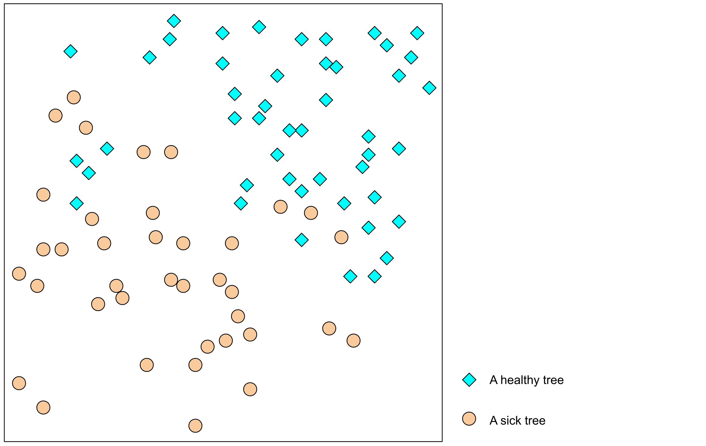
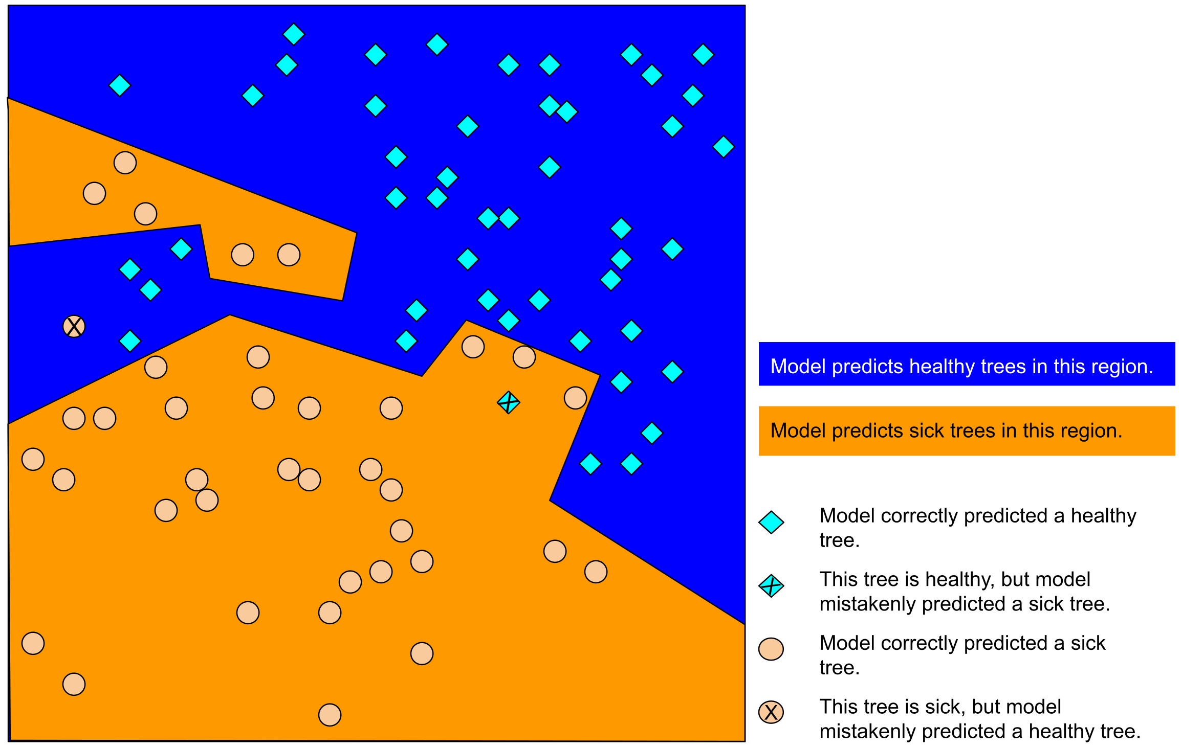
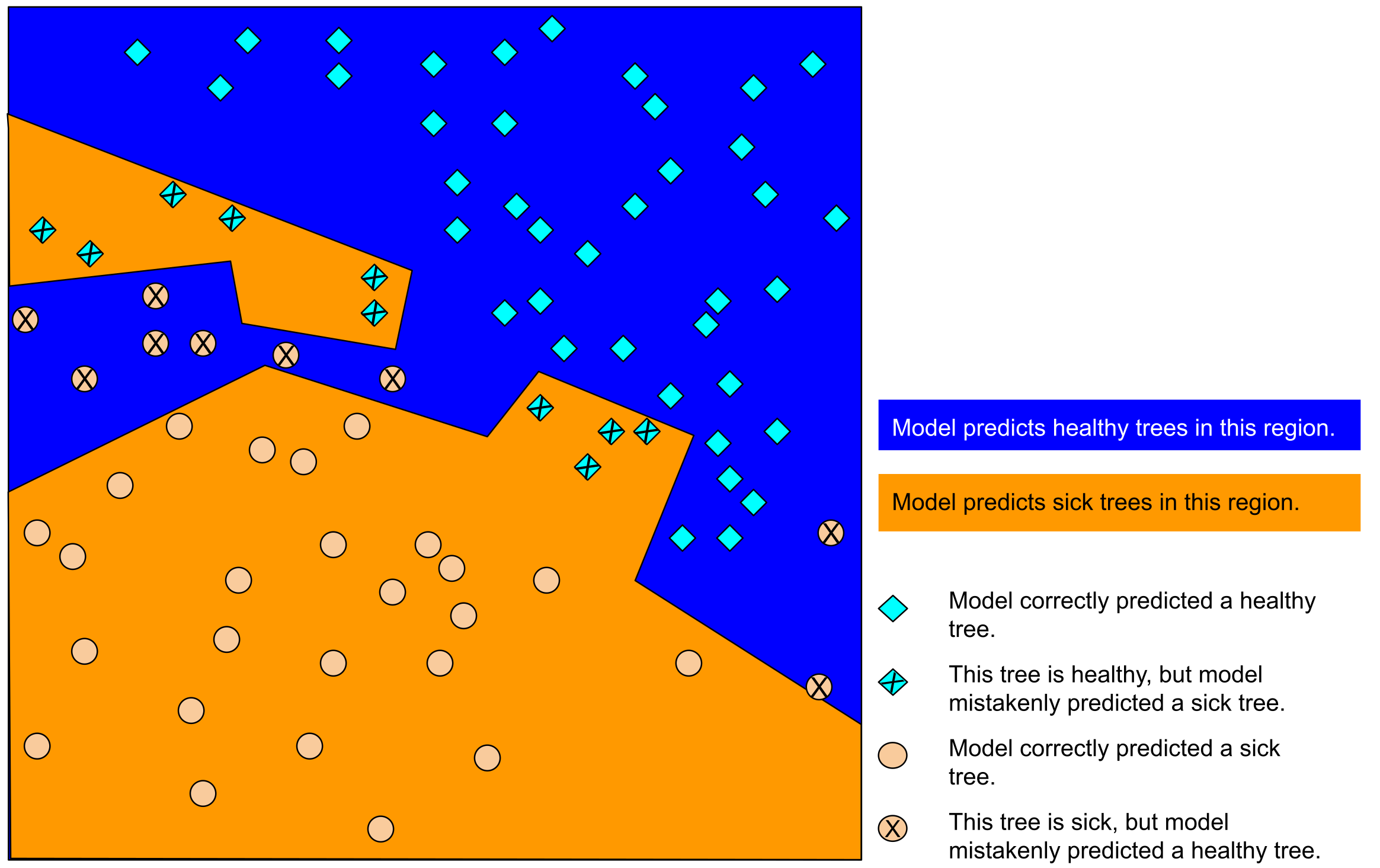
The three diagrams show training examples, a fitted boundary and new examples evaluated against it. A complicated boundary can follow the training points closely yet classify new points badly. This is overfitting. Underfitting is the opposite difficulty: the model fails to capture useful structure even in the training data. The goal is useful performance on the situations the system will encounter, not merely on remembered examples.
Training data fits parameters. Validation data helps choose settings and models. A test set supplies a later assessment; repeatedly choosing changes because they improve that same test score weakens its independence. Data leakage occurs when information unavailable at real prediction time influences development or evaluation. A duplicated image appearing in both training and test sets is a simple example.
These figures are from Google’s Machine Learning Crash Course, under CC BY 4.0, rasterized and resized from the source. Their lesson is to compare training behavior with genuinely new cases.
For sensor or video data, adjacent samples may be strongly related. Randomly splitting individual frames can place almost identical scenes on both sides. A deployment on a new machine, person or future period may need separation by that unit instead. An evaluation must reflect the actual question, including plausible changes in the environment.
Check: A model is perfect on training images. What essential evidence is still missing?
Its performance on independent, representative new images, including relevant failure cases. Training accuracy alone cannot establish generalization.
8. From a biological analogy to a numerical unit
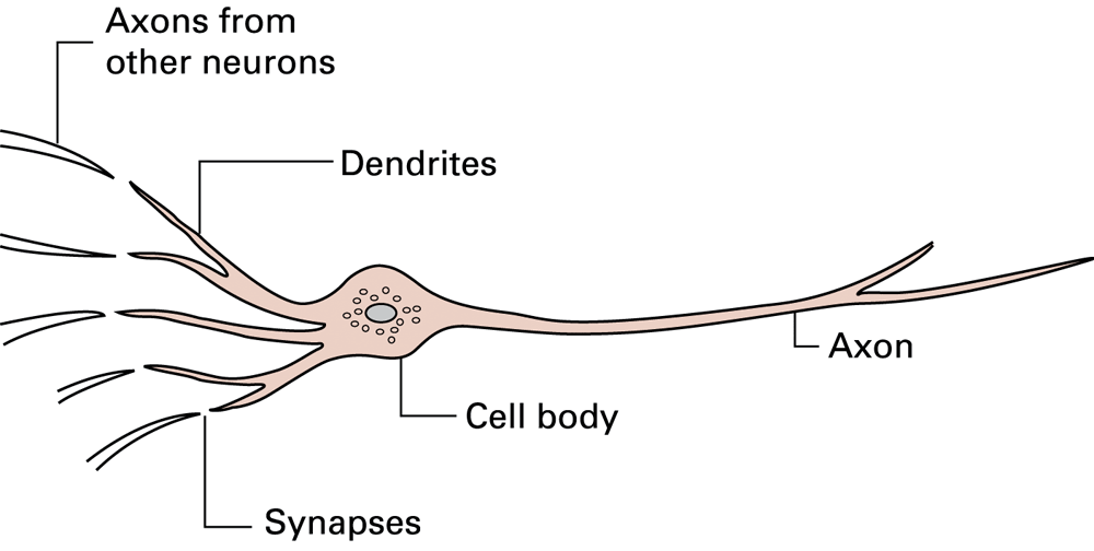
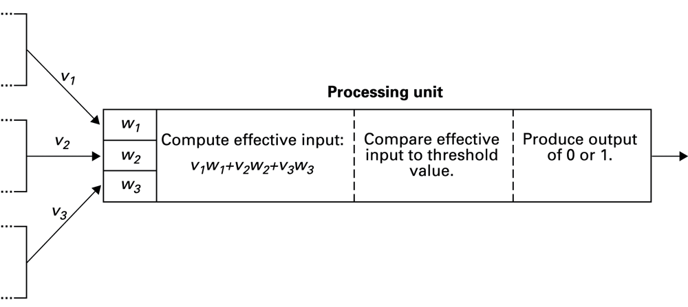
Artificial neural networks borrow an idea of interconnected processing units. They are mathematical models, not complete simulations of brains. A basic unit combines inputs using weights, adds an optional bias and applies an activation function. The output depends on numerical values and the activation rule, not only on which units are connected.
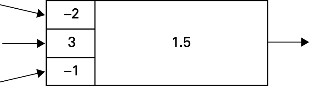
The original threshold example uses weights −2, 3 and −1 with inputs (0,1,1). The weighted sum is −2×0 + 3×1 −1×1 = 2. Its stated rule outputs 1 when the sum exceeds 1.5, so this input produces 1. A threshold of 1.5 can equivalently be represented by a bias of −1.5 and a threshold at zero, provided the comparison convention is preserved.
Check: For inputs (1,1,0) in the same unit, what is the output?
The sum is −2 + 3 = 1. It does not exceed 1.5, so the output is 0.
9. Layers and nonlinearities expand what can be represented
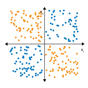
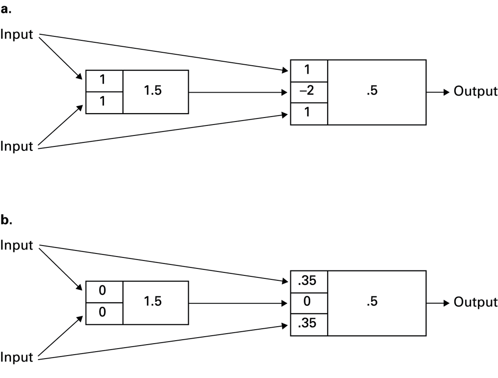
A single straight boundary cannot separate every arrangement of classes. Hidden units and nonlinear activations can combine simpler computations into more complex boundaries. If a sequence of layers were purely linear or affine, it could be combined into one affine transformation; adding layers alone would not supply the same expressive benefit.
The original XOR networks show why a connection diagram is incomplete without weights and activation rules. XOR should produce 1 for unequal binary inputs and 0 for equal ones. Two networks with similar wiring can behave differently. Check their computed outputs instead of assuming that a familiar shape implements the intended function.
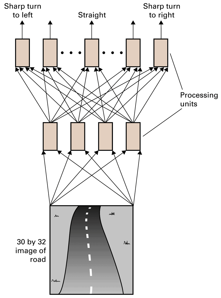
ALVINN is a historical illustration of learning steering from camera information. The figure connects measurements, hidden computations and an output choice; it is not evidence that a modern autonomous-driving system consists of this network alone. The nonlinear-boundary figure is from Google ML Crash Course, CC BY 4.0.
During training, a forward pass computes predictions and loss. Backpropagation applies the chain rule to calculate gradients through differentiable computations. An optimizer uses those gradients to adjust parameters. Backpropagation computes sensitivity; the optimizer determines the update. Improvement on one example can worsen another, which is why evaluation must consider many examples.
Check: Does a network diagram with the right number of layers prove that XOR is computed correctly?
No. The numerical parameters and activation functions determine the mapping. Test all four binary input pairs.
10. Generating content is not retrieving a guaranteed fact
A classifier predicts a category; a generative model produces a sample such as text or an image. In an autoregressive language model, the next token is predicted from the preceding context. A token may be a word, part of a word or another unit of encoding. Generation repeatedly selects a token and adds it to the context.
| Context | Candidate | Probability |
|---|---|---|
| The kettle contains hot | water | 0.60 |
| Same context | tea | 0.25 |
| Same context | air | 0.10 |
| Same context | other tokens combined | 0.05 |
The probabilities sum to one. A decoding procedure may choose the most likely token or sample from a modified distribution. Different decoding choices can produce different continuations from the same model. A plausible continuation can still be false: the training objective and generation process do not by themselves certify factual accuracy.
Diffusion models illustrate a different family of generative methods: they learn a process related to reversing added noise to construct samples. Do not describe every generative model as next-token prediction. The appropriate account depends on the model architecture and training objective.
Check: If “water” has probability 0.60 in this illustration, does the model know that a real kettle contains water?
No. The number describes a candidate continuation under the illustrative context. It does not verify the state of a physical kettle.
11. Context, attention and application tools
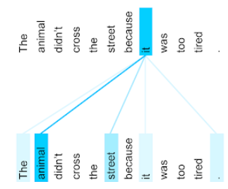
Attention computes weighted combinations of information from positions in a sequence. The diagram uses a sentence about an animal and a street to illustrate contextual relationships. Attention is a numerical computation; its name should not be interpreted as proof of human-like awareness. This Google ML Crash Course diagram is CC BY 4.0; see the transformer introduction and the original Attention Is All You Need paper.
A deployed application can add document retrieval, calculators, databases or other tools around a model. Retrieved information can supply relevant context, but does not guarantee that the response uses it correctly. Likewise, generating text that looks like a tool result is different from actually executing a tool and receiving its output.
Evaluate the complete application: the retrieved sources, requested actions, returned results and final claims. A base model, a retrieval system and an interface have separate responsibilities. For factual questions, inspect the evidence behind an answer rather than treating fluent wording as evidence.
Check: If a chatbot cites a document title, has it necessarily retrieved and checked that document?
No. Verify that the document exists and supports the claim. A generated reference can be inaccurate even when formatted convincingly.
12. A single accuracy score can hide important errors
| Actually defective | Actually sound | |
|---|---|---|
| Predicted defective | 16 | 3 |
| Predicted sound | 4 | 77 |
There are 16 true positives, 3 false positives, 4 false negatives and 77 true negatives. Accuracy is (16 + 77)/100 = 93%. Recall for defects is 16/(16 + 4) = 80%: the system misses one fifth of the actual defects. Precision is 16/(16 + 3), approximately 84.2%: that fraction of its defect warnings is correct.
Which errors matter depends on the task. False alarms consume inspection effort; missed defects can allow faulty parts through. Changing a decision threshold may change the trade-off. For definitions and further examples, use Google’s classification metrics lesson.
If only one part in a hundred were defective, predicting “sound” for everything would reach 99% accuracy while finding no defects. Also inspect performance across relevant conditions: lighting, device types, operating ranges and groups of users. Overall performance can hide a weak subgroup or a failure after conditions change.
Reliability also depends on the surrounding process: what happens when the system is uncertain, how people review outputs and how errors are detected after deployment. The NIST AI Risk Management Framework offers a broader resource for considering system risks and evaluation responsibilities.
Check: Is 93% accuracy sufficient to conclude that the inspection system is ready?
No. We need the error breakdown, representative test conditions, the costs of different errors and a suitable operational review process.
13. Access rules and storage representations are different
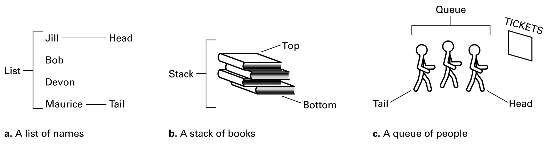
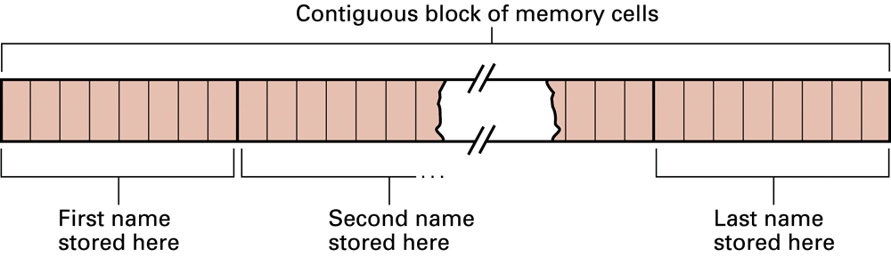
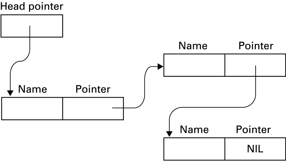
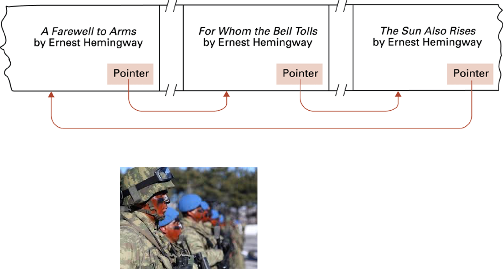
The second strand of this week builds on Week 11 structures and Week 9 pointers. An array keeps elements contiguously and supports direct indexing. A linked list stores a successor reference in each node; the logical order follows links and need not match physical memory order. The original bookshelf analogy shows one physical arrangement supporting another logical ordering.
A list describes a sequence. A stack specifies last-in, first-out access; a queue specifies first-in, first-out access. A stack or queue can be implemented with an array or linked nodes. Do not confuse the access rule with one particular storage diagram.
The useful comparison is operation-specific. Arrays provide direct access to an index and often good locality. Inserting into the middle may require moving elements. A linked list can change a few links once the relevant node is known, but locating that node still costs a traversal in a simple singly linked list. Links also consume storage and require lifetime management.
Check: Is insertion into a linked list always constant-time from the moment a user supplies an ID?
No. Searching for that ID may take linear time. Relinking after a known valid predecessor is the short operation.
14. A node is a record with a link
typedef struct Node {
    int event_id;
    int value;
    struct Node *next;
} Node;
The fields describe one event; next points to the successor node or is NULL at the end. The structure contains a pointer to its own type, not another complete Node object embedded recursively. A complete embedded copy would require a size that never ends. The tag struct Node is available for declaring the self-referential pointer.
Node c = {103, 30, NULL};
Node b = {102, 20, &c};
Node a = {101, 10, &b};
Node *head = &a;
These are ordinary local objects. They remain valid while their enclosing block is active. No malloc is involved, so they must not be passed to free. The head pointer is the entry point, not an extra data node. Following next yields 101, 102, 103 regardless of where the compiler places the objects in memory.
Check: Can a function safely return a pointer to a local Node that ceases to exist when the function returns?
No. The pointer would no longer designate a live object. The list needs an ownership and lifetime arrangement that outlasts its use.
15. Follow the links and stop before dereferencing NULL
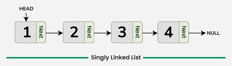
void print_list(const Node *p)
{
    while (p != NULL) {
        printf("%d: %d\n", p->event_id, p->value);
        p = p->next;
    }
}| Iteration | p points to | Output | Next p |
|---|---|---|---|
| 1 | a | 101: 10 | &b |
| 2 | b | 102: 20 | &c |
| 3 | c | 103: 30 | NULL |
| Stop | NULL | Nothing | No dereference |
The condition is checked before member access. An empty list starts with NULL and prints nothing. Advancing the local traversal pointer does not move the nodes or change head in the caller. const prevents changing node members through p in this function, while p itself can still advance.
This loop assumes a finite valid chain ending in NULL. A cycle can make it repeat indefinitely; a dangling pointer can make member access invalid. A termination condition does not prove the data structure satisfies the conditions needed to reach it.
Check: If p = p->next is omitted, what happens for a nonempty valid list?
The pointer never advances, so the first node is printed repeatedly. The condition remains true.
16. Preserve the successor before redirecting the link
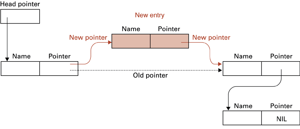
Node x = {104, 40, NULL};
x.next = a.next;
a.next = &x;
Initially a points to b. First, x receives the old successor, b. Then a is redirected to x. The resulting sequence is 101, 104, 102, 103. The nodes do not have to move. This example assumes x is a distinct live node that is not already in the chain.
Reversing the assignments is a real defect: after a.next = &x, reading a.next obtains x, not b. Assigning that value to x.next creates a self-loop and loses the original route to b. Drawing the arrows after each statement is often more effective than rereading both lines as one vague “insert” operation.
Check: For a list A → B, what is wrong with A.next = &X followed by X.next = A.next?
The second assignment sets X.next to X. Save B as X’s successor before changing A’s link.
17. Unlinking changes reachability, not object lifetime
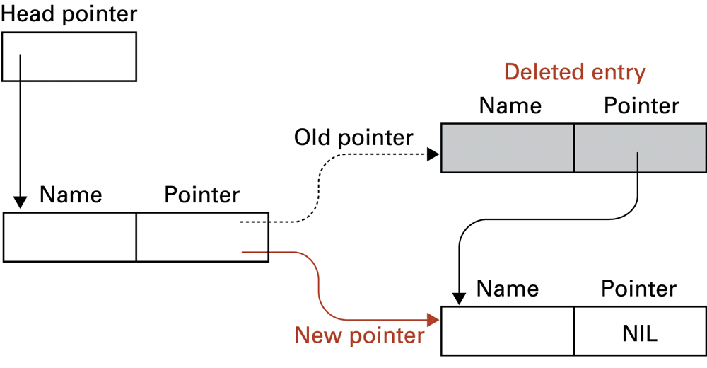
Node *victim = x.next;
if (victim != NULL) {
    x.next = victim->next;
    victim->next = NULL;
}
After the insertion above, x.next is b. Redirecting x to b’s successor bypasses b, leaving 101, 104, 103. Clearing b’s next makes its detached state explicit. The object b still exists. Other pointers might still refer to it, and this operation has not released storage.
Node *pop_front(Node *head)
{
    if (head == NULL) return NULL;
    Node *rest = head->next;
    head->next = NULL;
    return rest;
}
/* Caller: head = pop_front(head); */
Removing the first node changes the entry point, so the caller must use the returned head. The helper detaches but does not free the old first node. For these local objects that is appropriate. With allocated nodes, retain the removed pointer if cleanup is needed and define who owns it. A helper that loses the only pointer to allocated storage without releasing it would leak memory.
Check: Why must this example not call free(victim) when victim points to b?
b is a local object, not storage returned by a compatible allocation function. Unlinking it does not change how its storage was obtained.
18. Pointer correctness needs explicit invariants
| Mistake | Consequence | Question to ask |
|---|---|---|
| Dereference NULL | Invalid member access | Was the pointer checked first? |
| Lose the old successor | Remaining nodes become unreachable | Was the link saved before redirection? |
| Create a cycle | Traversal may not finish | Does every path reach the intended end? |
| Use an expired object | Dangling pointer | Is the node still alive? |
| Free the same object twice | Invalid memory operation | Who owns cleanup? |
For a simple list, maintain a live head or NULL, valid successor links, an intended termination point and a clear ownership policy. These are invariants: properties that operations must preserve. A function can be locally short and still be wrong if it breaks the larger structure.
The lecture uses known-lifetime local nodes so the link changes are visible without allocation machinery. Lab 11 supplies allocation and cleanup support where needed. Extended memory-management implementation is not added to the exercise. Diagram the empty, singleton, head-removal and middle-removal cases separately.
Check: Does checking head != NULL prove that every later next pointer is valid?
No. It only checks that head is not null. The rest of the chain still depends on correct construction, lifetime and updates.
19. Stacks and queues organize when an item is used
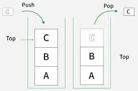
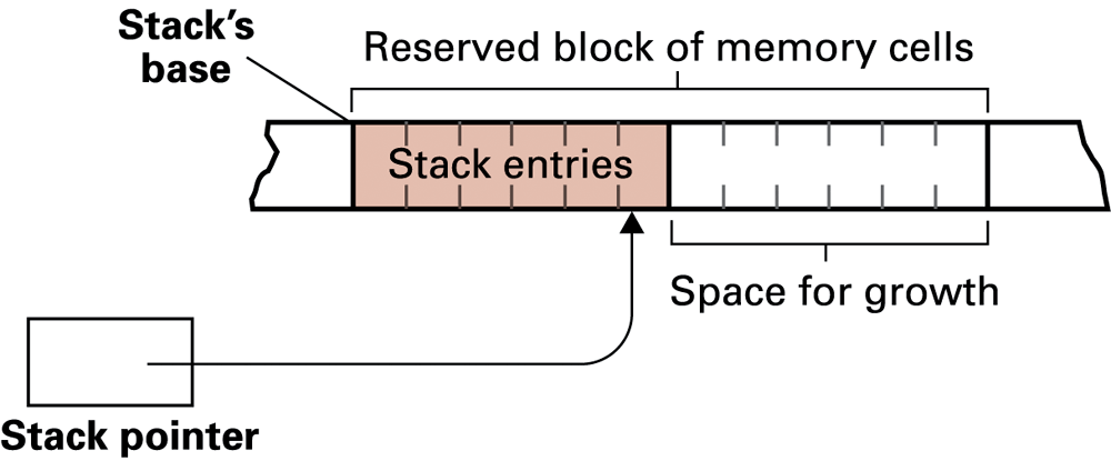
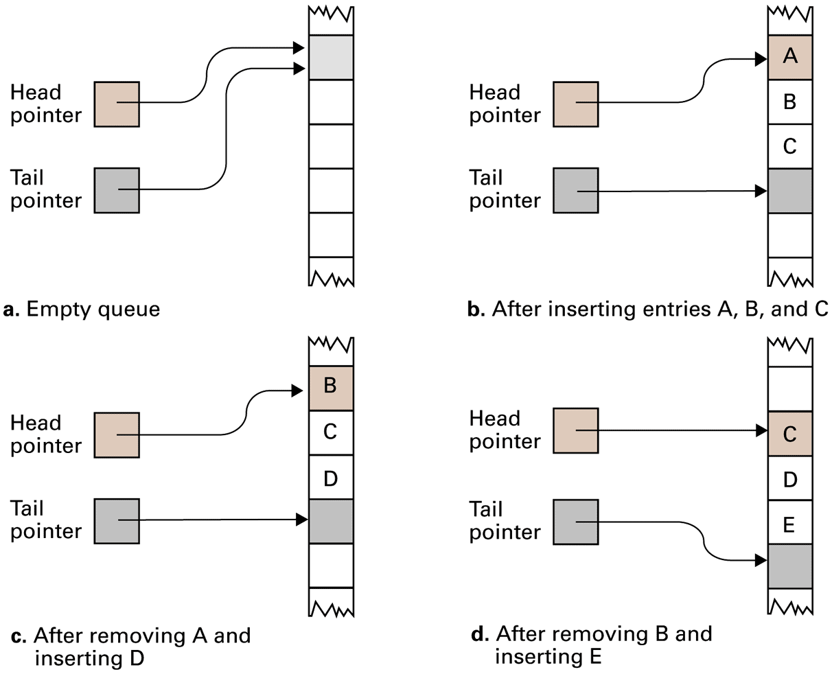
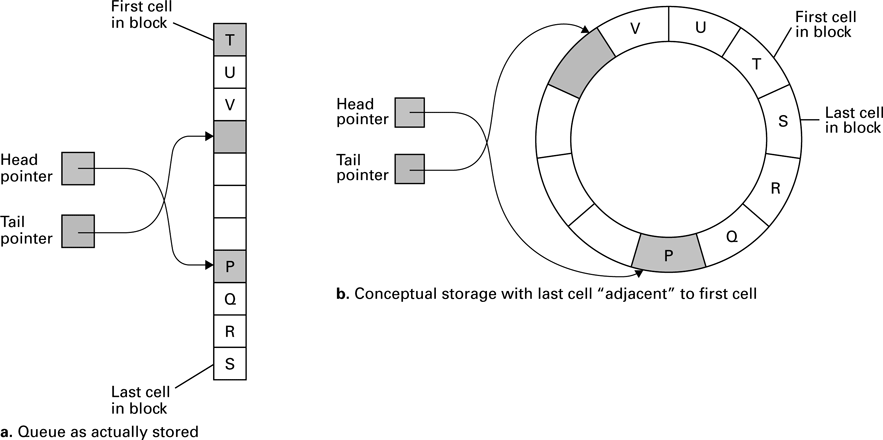
A stack pushes and pops at the same end, so the most recently added item is removed first. It suits nested work and returning to a previous state. A queue adds at one end and removes at the other, so earlier items leave first. It suits waiting tasks or buffered events. These rules are independent of whether the implementation uses nodes or an array.
In a bounded circular queue, indices wrap around to reuse array slots. Under a zero-based convention with positive capacity C, advancing an index can use (index + 1) % C. Equal head and tail indices need an additional convention to distinguish full from empty: for example, an explicit count, a full flag or reserving one unused slot. State the chosen convention before tracing it.
Check: With capacity 4, an explicit count and next-write index 3, where does that index go after one insertion when space exists?
It wraps to (3 + 1) % 4 = 0, and count increases by one. The exact meaning of head/tail names depends on the stated convention.
20. A hierarchy needs more than one successor
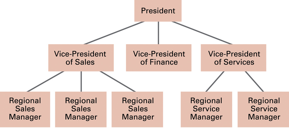
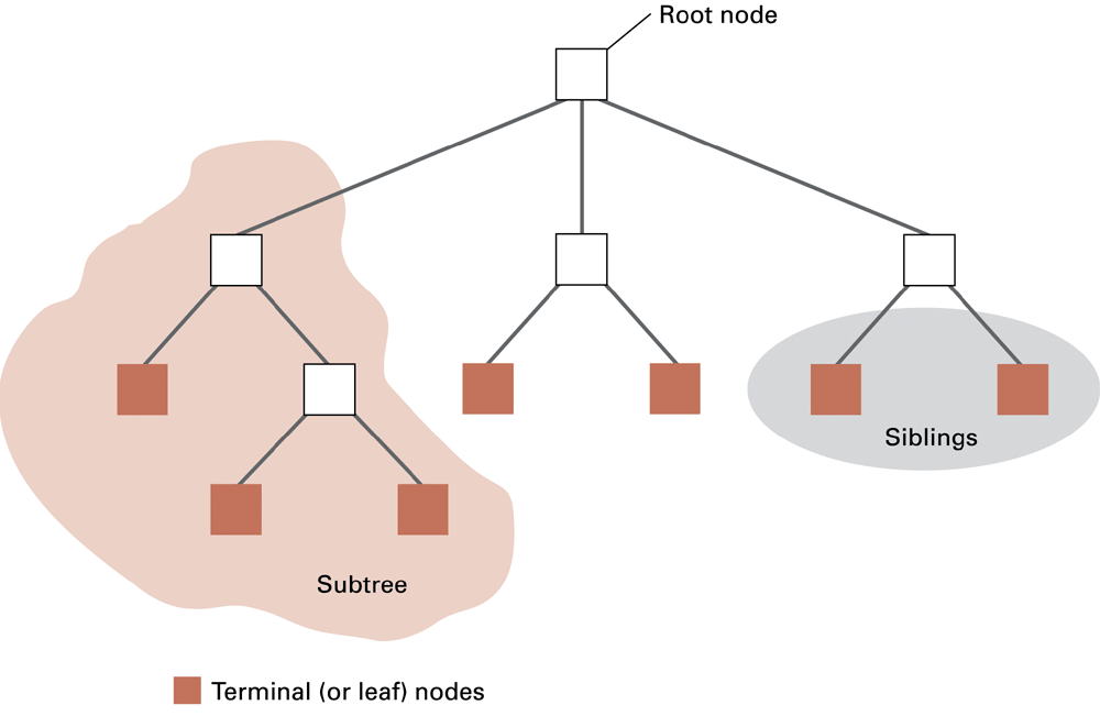

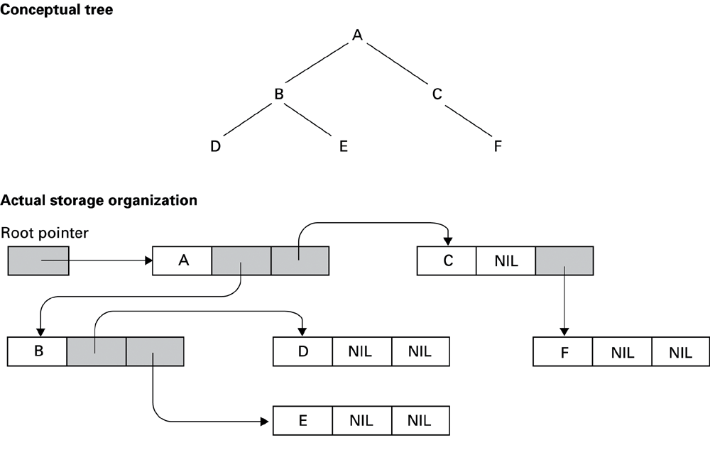
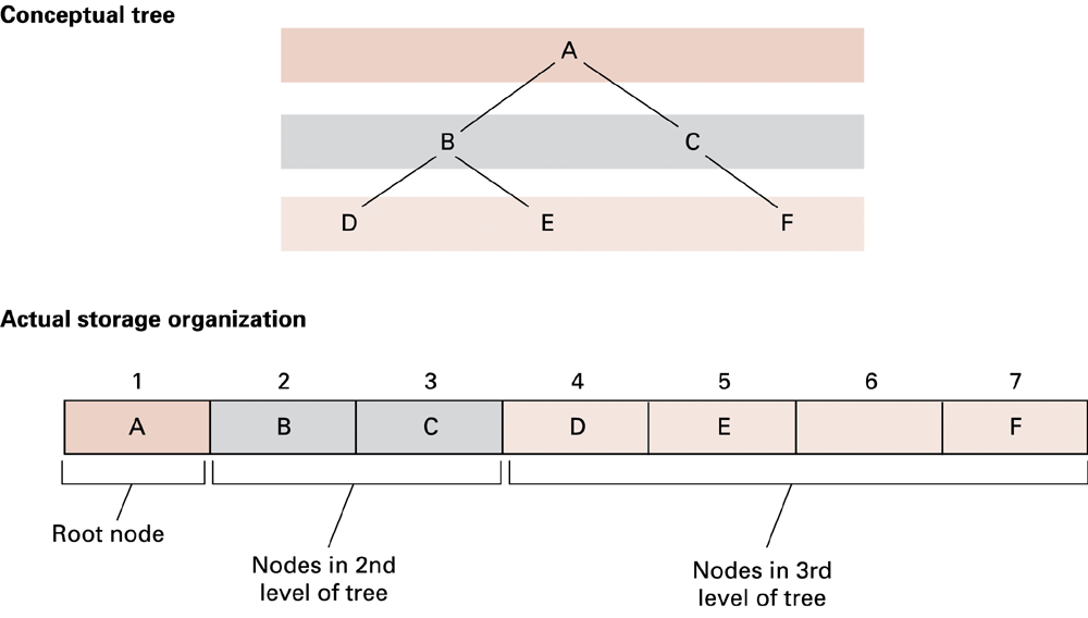
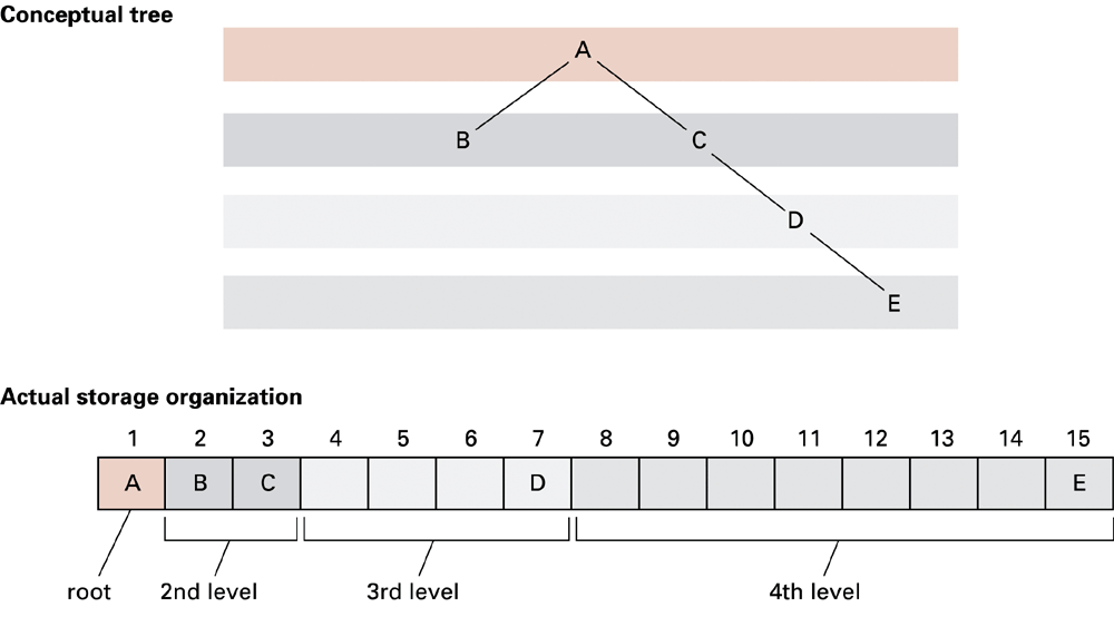
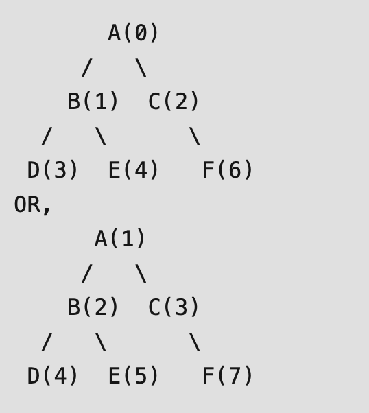
A tree expresses hierarchical relationships: a root, parent–child links and leaves with no children. A binary-tree node has at most two children. “Binary” alone does not imply search ordering. A binary search tree adds an ordering rule relating keys in the left and right subtrees to the node’s key, including a policy for duplicates.
Pointers can represent children explicitly. An array can encode their positions instead. For a zero-based complete-tree layout, children of i are 2i + 1 and 2i + 2; for a one-based layout they are 2i and 2i + 1. Inspect which convention a source figure uses before applying formulas. Sparse trees can waste many positions in such an array representation.
A doubly linked list adds a predecessor link; a graph can represent more general connections and cycles. These are recognition and comparison topics here. A graph is not automatically a tree, and following its links without a visited-state policy may revisit nodes.
Check: Does having two child pointers guarantee that a tree supports ordered search?
No. The key-ordering invariant must also hold. The representation alone does not enforce it.
21. Search, traversal and insertion have different goals
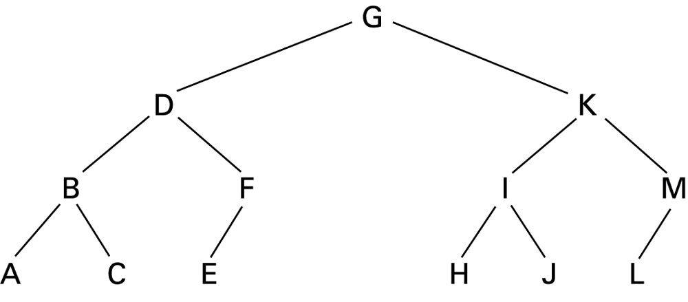
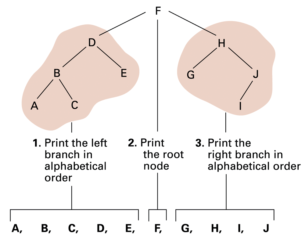
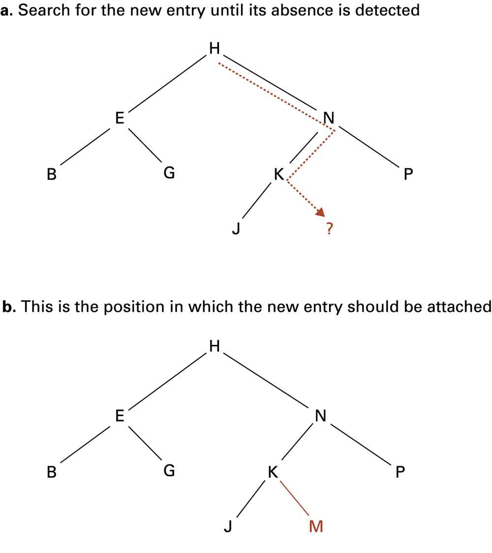
Week 8 explained why a balanced ordered tree can reduce the number of comparisons. Here inspect how the nodes and links store that ordering. Searching chooses a subtree from a comparison; visiting every node is a different operation. A highly unbalanced search tree can behave like a long chain, so binary branching is not by itself a logarithmic-time guarantee.
In-order traversal visits the left subtree, then the node, then the right subtree. It yields sorted keys for a binary search tree, subject to its duplicate convention. It visits any ordinary binary tree in that order too, but the resulting keys need not be sorted if the search-tree invariant is absent.
Insertion follows comparisons to an appropriate empty child position and links in a new node. The original M example makes the change visible. The search and insertion pseudocode is retained later for reference; implementing a tree is not part of this week’s list lab.
Check: Can an in-order traversal sort arbitrary values in an arbitrary binary tree without changing that tree?
No. It reports the values in traversal order. Sorted output depends on an ordering invariant already present in the tree.
22. What to carry into recitation and Lab 11
For AI, practice explaining where a decision comes from: an explicit rule, a searched alternative or learned parameters. State the evaluation data and the kinds of errors a score hides. For C, draw the nodes and update one arrow per statement. These are complementary forms of reasoning about a system’s behavior.
Lab 11 remains PC-focused: traverse or modify a supplied singly linked list and diagnose a familiar defect. Prepared records and allocation/cleanup support protect the focus on links. Live Arduino is optional. No tree, graph or standalone debugger implementation is required. Week 11 structures and the earlier pointer material are the prerequisites.
Check: What should be checked after inserting a node, beyond seeing the new ID once?
Verify the complete expected order, retention of the remaining nodes, termination and valid node lifetimes. One printed ID does not prove that the list is intact.
23. Optional: the complete original search trace
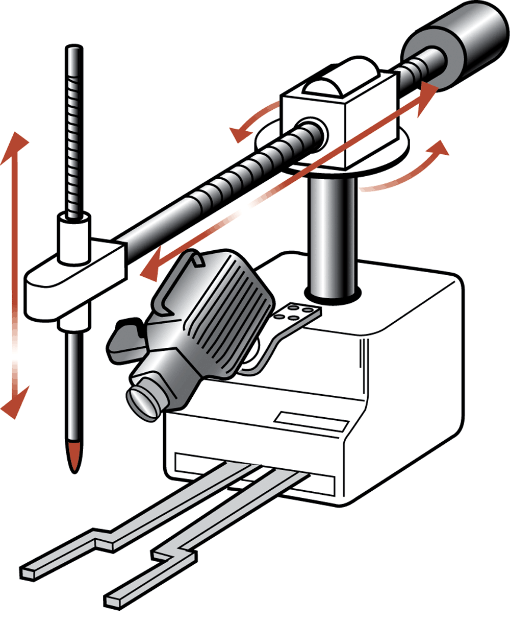
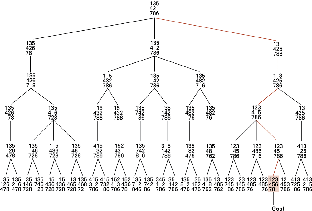
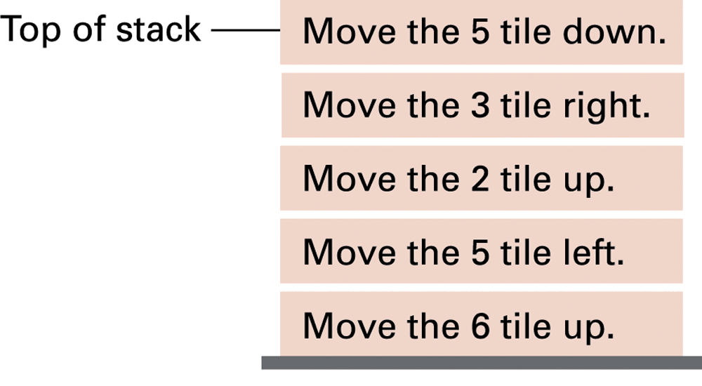
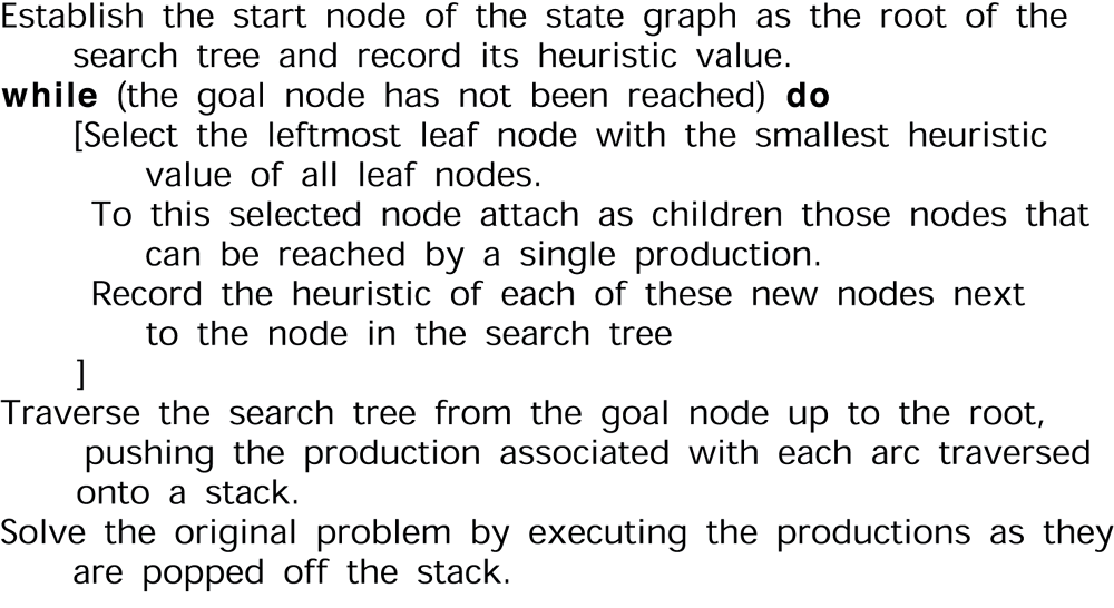
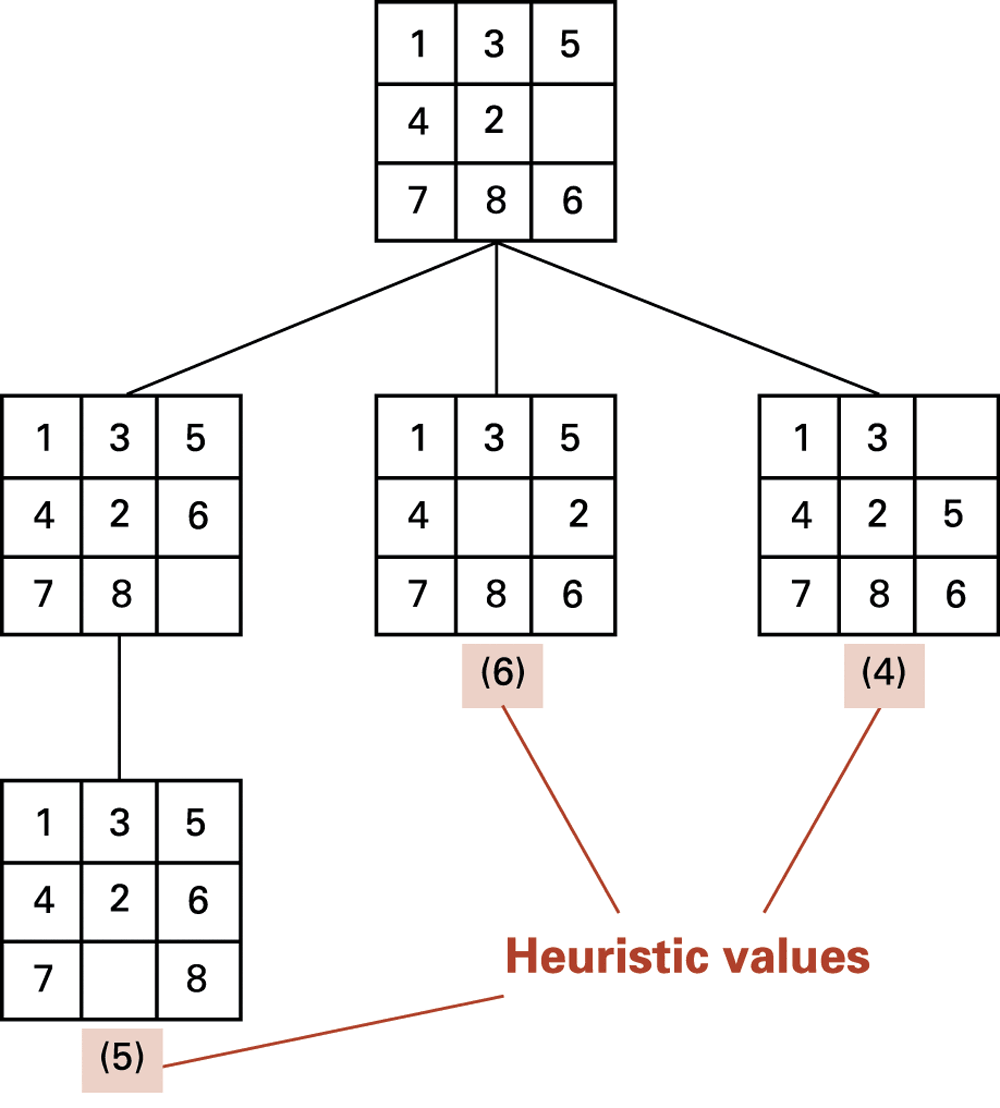
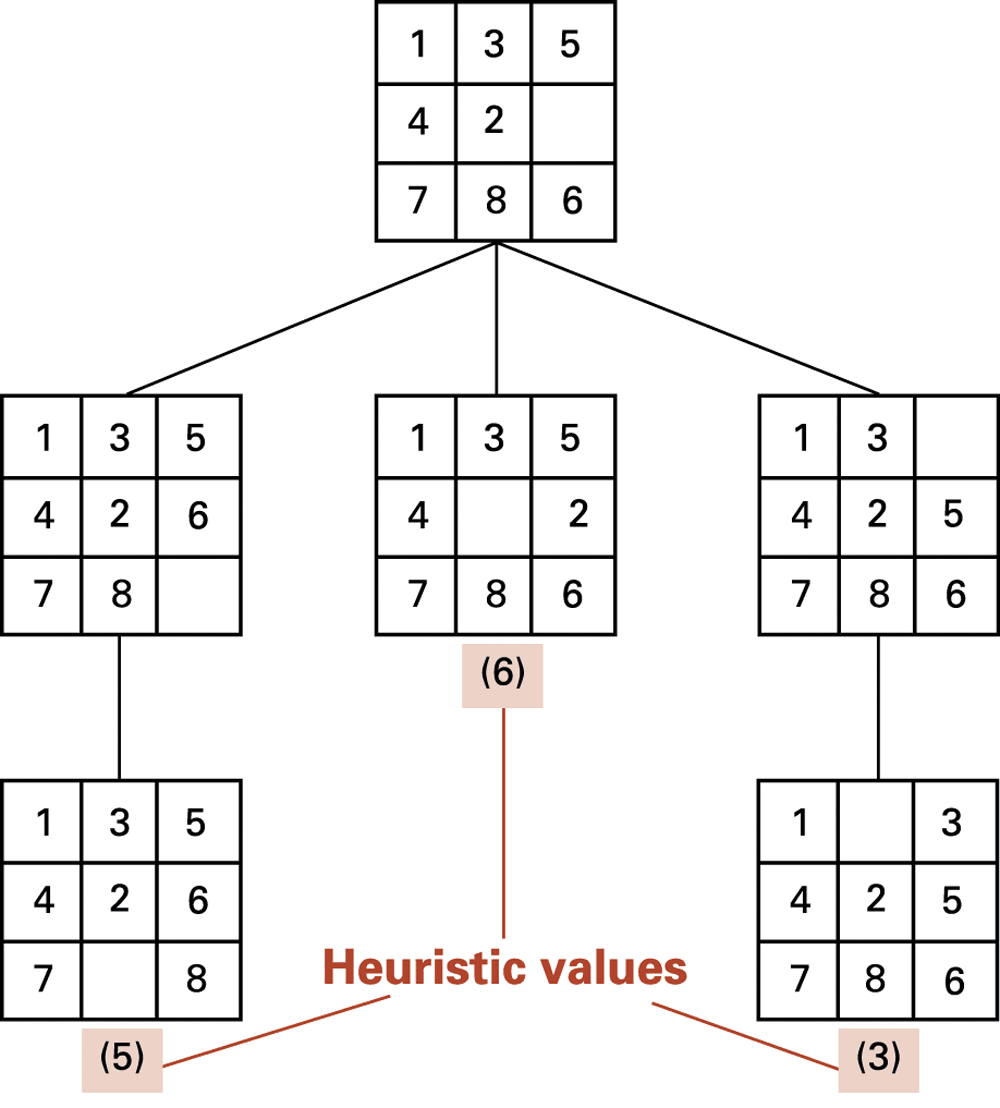
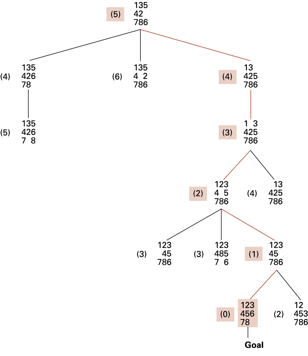
The original sequence links perception, a puzzle representation, candidate expansion and a stored action sequence. Follow the indicated top of the action stack. In the heuristic trace, compare newly generated candidates with those still waiting; choosing a promising branch does not make the other candidates disappear. The procedure prioritizes h alone, so its name here is greedy best-first search, not A*.
Check: Does a successful illustrated search prove that the procedure always finds a shortest solution?
No. It proves what happened in that example. A general optimality claim needs the algorithm’s assumptions and a separate argument.
24. Optional: weight changes and associative memory
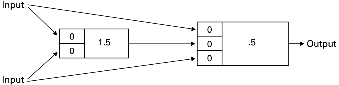
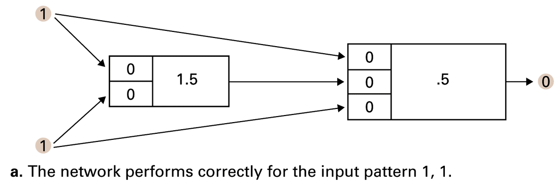
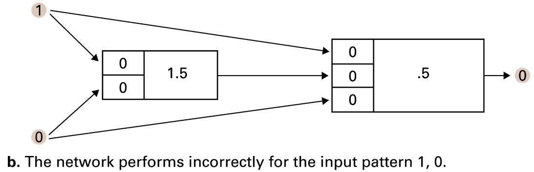
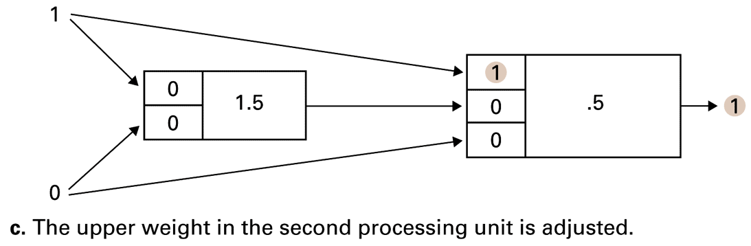
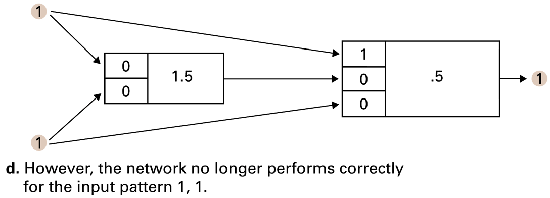
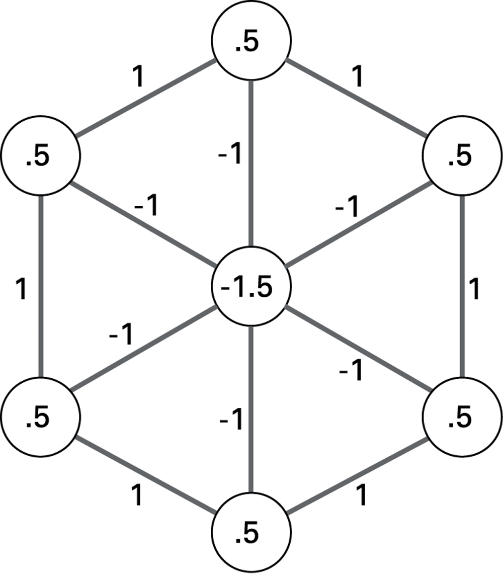
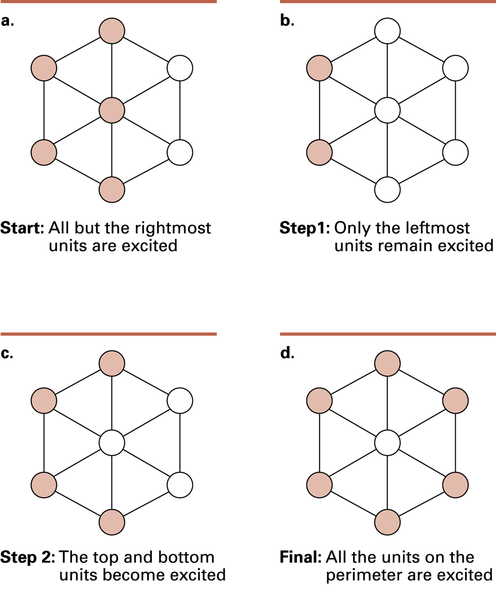
Trace the network output before and after each pictured adjustment. Correcting one XOR input can disturb another, so one successful example is not a completed learning task. Evaluate the whole intended truth table. The associative-memory figures then illustrate a different historical architecture that moves through configurations toward a stored pattern. Do not identify that settling process with autoregressive next-token generation.
Check: If a changed weight fixes one previously wrong input, is it safe to stop testing?
No. Recheck the other inputs. Shared parameters influence more than the example used to choose the change.
25. Optional: original structure procedures

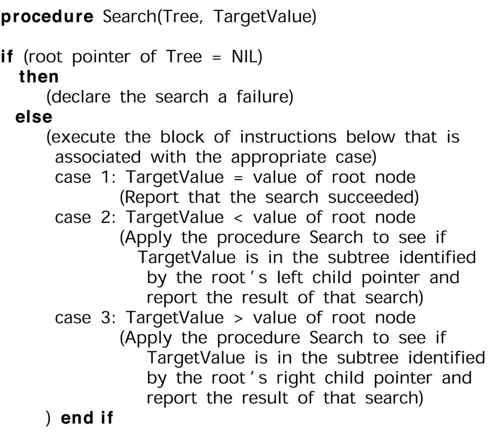
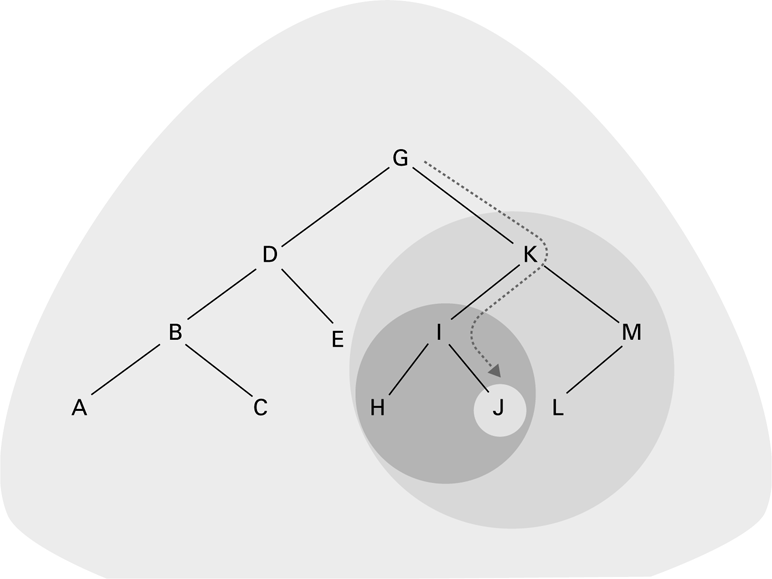
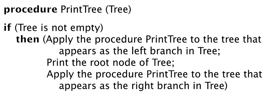
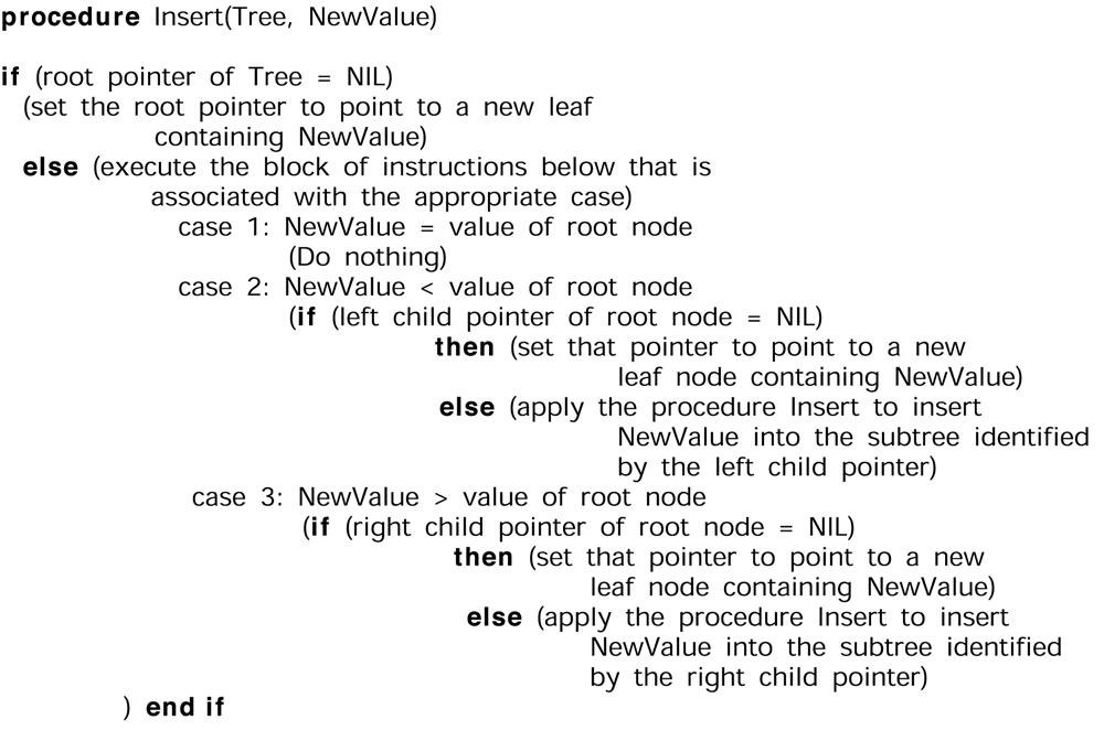
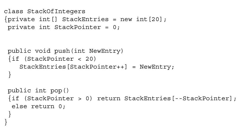
The original traversal and tree algorithms are retained for enlarged restudy. Read their stopping conditions before their recursive or iterative steps. The C traversal in the main text tests the pointer before accessing a member. The original stack class uses Java/C# notation for comparison; class syntax is not a requirement for the C examples.
Check: What is the stopping case for a recursive traversal of a pointer-based binary tree?
An empty subtree, usually represented by NULL. It should return without accessing node fields.
26. Sources and further study
The reading follows the accepted 99-slide Week 12 deck and preserves all of its teaching images. Original AI figures come from the supplied Brookshear tenth-edition slides; the accompanying book is the twelfth Global Edition. Figure numbering differs between editions. Data-structure images come from the instructor’s original collection. The local figure manifest records exact source parts and inherited notes.
- Brookshear & Brylow, Computer Science: An Overview, 12th Global Edition, Chapter 11, for AI foundations; consult its data-structure coverage alongside the original diagrams.
- SRI: Shakey, IBM: Deep Blue, and Google DeepMind: AlphaGo for the pictured historical systems. Photographs retain source attribution; no open-license claim is made for them.
- Google ML Crash Course: overfitting and classification metrics for generalization and worked evaluation.
- Google ML Crash Course: neural networks and transformers. Reproduced Google diagrams use CC BY 4.0; SVG originals were rasterized/resized.
- Vaswani et al., Attention Is All You Need and Ho et al., Denoising Diffusion Probabilistic Models: optional primary papers for the two model families, not required mathematics for this lecture.
- NIST AI Risk Management Framework for broader evaluation and risk questions.
- WG14 N1570, public C11 committee draft, for structure members, pointers and storage duration. This is a reference, not the C17 standard or required cover-to-cover reading.
A useful review task is to compare two kinds of graph: a search-state graph and a linked data structure in memory. In each case explain what a node means, what a link means, why cycles matter and what information an algorithm must retain. Similar-looking arrows can represent very different relationships.