CSE 101 · WEEK 08 · READING
Algorithm efficiency and multidimensional arrays
Why ordering can save work, how sorting builds order, and how arrays organize a batch of readings.
Predict the traces before opening the Check answers. The theoretical discussion stands on its own; the C examples make selected mechanisms concrete. The final puzzle and recursive-search sections are optional references. Lab 7 begins with a one-dimensional traversal before a small two-dimensional extension; no sorting benchmark or extra hardware is required.
1. An algorithm needs an agreed vocabulary
An algorithm describes a method for producing a required result from an input. It can be represented in words, a flowchart, pseudocode or pictures. A program expresses a method in a particular language. The problem, the method and the program are related, but they are not interchangeable: different algorithms can solve the same problem, and the same algorithm can be implemented in different languages.
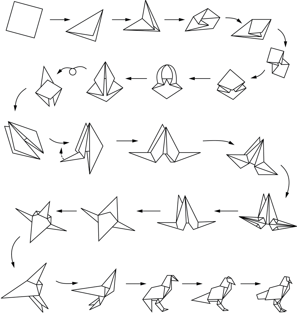
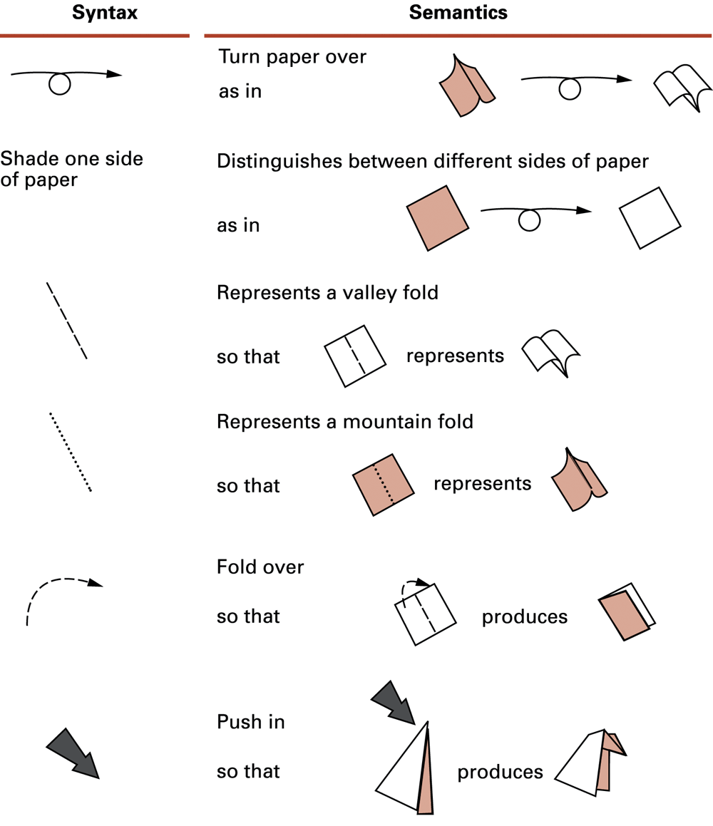
The origami reader must know what a fold line, arrow and shaded side mean. Likewise, “compare the middle item” requires an agreed ordering and a way to identify the middle. Choosing suitable primitives lets a long method be explained through a small vocabulary. A missing convention can make a seemingly clear instruction ambiguous.
Pólya’s problem-solving stages offer a useful discipline: understand the problem, devise a plan, carry it out and look back at the result. Work through a small instance before coding. State what counts as success, what inputs are allowed and what should happen when no solution exists. Looking back includes checking correctness and considering whether another representation would reduce the work.
Check: Does a detailed flowchart guarantee that a method solves the intended problem?
No. It can precisely describe the wrong method or rely on an unstated assumption. Compare the traced behavior with the required result and test failure cases.
2. Searching with a clear contract
Our search problem receives n accessible elements and a target. It returns a matching index or −1 when the target is absent. Require n to be nonnegative and no greater than the available length. Unless a stronger contract is stated, any matching index is acceptable when values repeat. An empty collection returns −1 without accessing an element.
Sequential search checks items in order until it finds a match or reaches the end. It needs no sorted order. For the array 18, 7, 31, 12 and target 31, the first two probes fail and the third succeeds. The returned index is 2, while the number of probes is 3. A position and an amount of work are different quantities.
| Index | Value | Action |
|---|---|---|
| 0 | 18 | Continue |
| 1 | 7 | Continue |
| 2 | 31 | Return 2 |
| 3 | 12 | Not examined |
For target 9 in the same collection, all four elements must be examined. After each unsuccessful probe, no examined element matches. This fact is preserved as the examined prefix grows. Reaching the end establishes absence under the contract; stopping early without a match would leave unexamined possibilities.
Check: What should happen for n = 0, even if the allocated array contains other values?
No elements belong to the requested search range. Return −1 and perform zero element probes.
3. Define the operation and the case
To compare algorithms, first decide what to count. Here a probe means inspecting one candidate element against the target. It is not necessarily one machine instruction or one C comparison. Binary-search code may test both equality and ordering during one probe.
| Case | Probes |
|---|---|
| First element matches | 1 |
| Last element matches | n |
| Target absent | n |
| Successful position uniformly distributed | (n + 1) / 2 on average |
The average follows from (1 + 2 + … + n) / n. It assumes a successful search and equal probability for every matching position. A workload with mostly unsuccessful searches, or frequent matches near the beginning, has a different average. “Average case” is incomplete without the distribution being assumed.
Operation counts explain scaling without depending on one stopwatch reading. Actual elapsed time also depends on the machine, implementation, memory behavior and the cost of comparing an element. Comparing long strings need not cost the same as comparing fixed-size integers. Use a model appropriate to the question and label its limits.
Check: For four equally likely successful positions, why is the average 2.5 probes rather than 2?
The possible counts are 1, 2, 3 and 4. Their average is 10/4 = 2.5. Individual executions use whole probes, but their mean need not be an integer.
4. Binary search uses order to eliminate possibilities
In ascending data, every element before a middle item is no larger, and every element after it is no smaller. If the target is smaller than the middle value, a match cannot lie in the right-hand part. If it is larger, a match cannot lie in the left-hand part. Binary search uses this ordering to discard a large region after each unsuccessful probe.
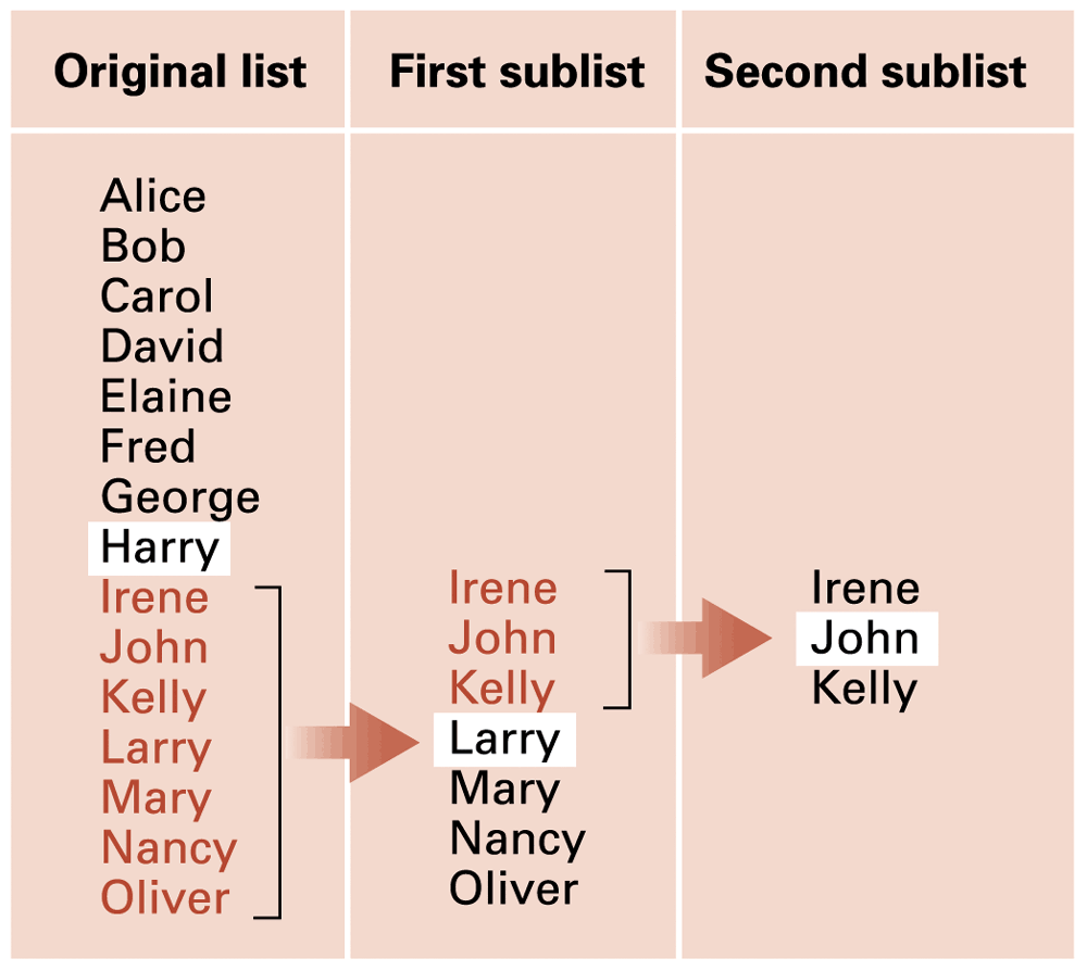
This reasoning fails on arbitrary unsorted data. For example, in 18, 7, 31, 12, observing that the target 12 is larger than 7 does not prove that every earlier item can be discarded according to a sorted-array rule. The method’s efficiency depends on a precondition. A fast answer from a violated precondition may be wrong.
| Candidate indices | Middle | Decision |
|---|---|---|
| 0…6 | index 3, value 18 | Keep 4…6 |
| 4…6 | index 5, value 31 | Return 5 |
For inclusive integer bounds lo and hi, use the middle index lo + (hi - lo) / 2. The division rounds down here because the difference is nonnegative. This expression also avoids forming the possibly overflowing sum lo + hi. When the middle is not a match, exclude it from the next candidate interval: use mid + 1 or mid − 1.
Check: Why is “look at the middle” insufficient as a complete binary-search description?
We also need sorted input, an interval convention, an update that excludes the tested middle, and a stopping rule. Without those, a method can discard a valid match or repeat the same interval forever.
5. The ordered tree makes branch elimination visible
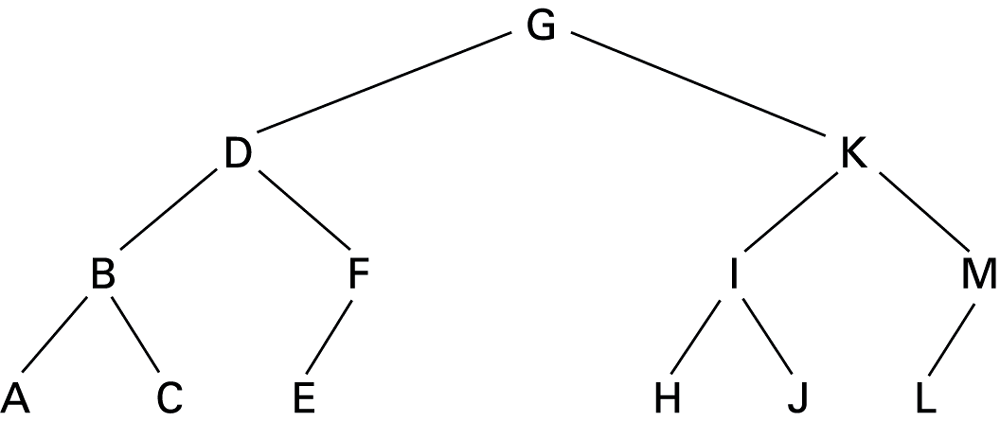
At G, J is larger, so the left subtree can be skipped. At K, J is smaller, so take the left branch. At I, J is larger, leading to J. Ordering justifies each eliminated branch. The diagram makes the central advantage visible: a comparison can remove many candidates rather than only one.
A binary search tree and binary search on an array are different representations. The tree stores relationships between nodes; the array algorithm computes midpoint indices. The pictured tree is not the exact decision tree of every midpoint convention, and binary search on an array does not require stored links.
The height of a tree affects its path lengths. A shallow, balanced tree supports short searches. A tree shaped like a long chain can require a linear number of visits despite satisfying the ordering rule. Thus “binary” describes branching possibilities, not an automatic guarantee of logarithmic performance for every stored tree.
Check: If the letters were stored in an ordered tree with only a right child at every node, would the search necessarily take about log₂ n visits?
No. The tree would be a chain. Searching near its end could visit all n nodes. The ordering is useful, but the shape controls the path length.
6. Absence, invariants and termination
| Candidate indices | Middle value | Next interval |
|---|---|---|
| 0…6 | 18 | 4…6 |
| 4…6 | 31 | 4…4 |
| 4…4 | 24 | 5…4: empty |
An interval with lo greater than hi contains no candidate indices. The algorithm reports not found; it does not read another element. Empty input begins in exactly this situation, with lo = 0 and hi = −1.
A useful invariant is: if the target exists in the original search range, a matching element remains in the candidate interval. Initially the whole range qualifies. Ordering justifies each reduction without losing a possible match. An unsuccessful probe also strictly reduces the number of candidates. The invariant supports correctness; the reduction supports termination. Both are necessary.
Updating lo to mid rather than mid + 1 can fail to make progress when mid equals lo. Similarly, an incorrect comparison can preserve the wrong half. Trace the smallest cases—empty, one item and two items—because a boundary error can be hidden by a longer successful example. CMU’s binary-search notes develop interval and invariant reasoning in more detail; interval conventions must be used consistently.
Check: Why is an invariant alone insufficient to prove that a loop finishes?
A loop could preserve a true statement while repeating the same state forever. We also need progress toward a finite stopping condition, such as a strictly shrinking candidate interval.
7. Logarithmic, linear and quadratic growth
For n = 2ᵏ − 1 sorted elements, binary search needs at most k middle-element probes. After a failed middle check in 15 elements, at most 7 remain, then 3, then 1. The longest route uses four probes. In general, for n ≥ 1, the inclusive search here uses at most floor(log₂ n) + 1 probes.
| n | Sequential search | Binary search |
|---|---|---|
| 15 | 15 | 4 |
| 255 | 255 | 8 |
| 1,023 | 1,023 | 10 |
| 1,048,575 | 1,048,575 | 20 |
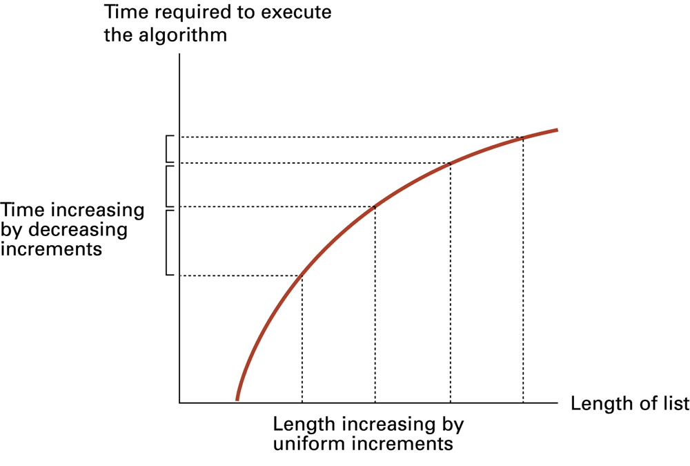
A doubling of a large input roughly doubles linear work but adds about one probe to binary search’s worst case. A quadratic method instead grows roughly fourfold when input size doubles. These descriptions concern behavior as input grows, not exact time on a particular computer.
| Tight class | Example | Effect of doubling input |
|---|---|---|
| Θ(1) | Read one known array element in the usual random-access model | No size-dependent increase |
| Θ(log n) | Binary search, worst case | About one more probe |
| Θ(n) | Sequential search, worst case | About twice the probes |
| Θ(n²) | Insertion sort, worst case | About four times the leading work |
Θ names a tight asymptotic growth class; O gives an asymptotic upper bound. Constants and smaller-order terms are suppressed, so 2n + 5 has linear growth. An upper bound need not be tight: linear work is also O(n²), but Θ(n) is more informative. Big O does not itself mean “worst case”; specify which case or cost function is being bounded.
Check: Does O(n²) tell you an exact number of seconds, or even that the algorithm always performs n² operations?
Neither. It is an eventual upper-bound statement up to a constant factor. Exact counts, machine speed and the chosen case require additional information.
8. Include preparation, memory and the workload
If data arrive unsorted and you need one answer, a sequential scan can be the sensible choice. Sorting adds work before a binary search can begin. If the same mostly unchanged data will be searched many times, that preparation can be shared across the queries. Updates may require further work to preserve order.
A simple illustrative model makes the trade-off explicit. Suppose sorting costs 1,000 work units, a scan costs 100 units per query and a binary search costs 7. For q queries, compare 100q with 1,000 + 7q. The prepared approach wins in this model when 93q exceeds 1,000, so from 11 queries onward. These are assumed compatible cost units, not a benchmark or universal crossover point.
Extra structures or copies consume memory but can avoid repeated computation or preserve original order. Iterative binary search needs only a fixed set of indices beyond the input. A recursive version retains call state; with shrinking intervals and no subarray copying, its depth is logarithmic. Copying each sublist introduces additional costs that are absent from the simple index model.
Hardware matters, but growth can outweigh it. At n = 100,000, a model requiring n² operations takes 100 seconds on a hypothetical machine performing 100 million model operations per second. A linear n-operation method takes 0.1 seconds on a machine performing only one million per second. The example isolates growth; it does not predict real timings.
Check: A report says “binary search used only seven probes” after sorting a new file for one query. What is missing from the comparison?
The preparation cost, along with any copying, update and memory costs relevant to the workload. Search probes alone do not measure the complete task.
9. Sorting must preserve the data as well as order it
Sorting rearranges entries according to a chosen key. The result must be ordered and contain the same entries with the same multiplicities. Replacing 7, 3, 5, 3 with 3, 3, 3, 3 produces an ordered sequence but destroys information. Correctness requires both properties.
For records, keep related fields together. Sorting only a column of names while leaving their associated marks in place pairs names with the wrong marks. Likewise, sorting sensor values changes their time order. Use a copy or another representation if later processing must preserve the original sequence.
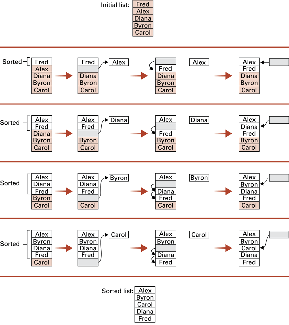
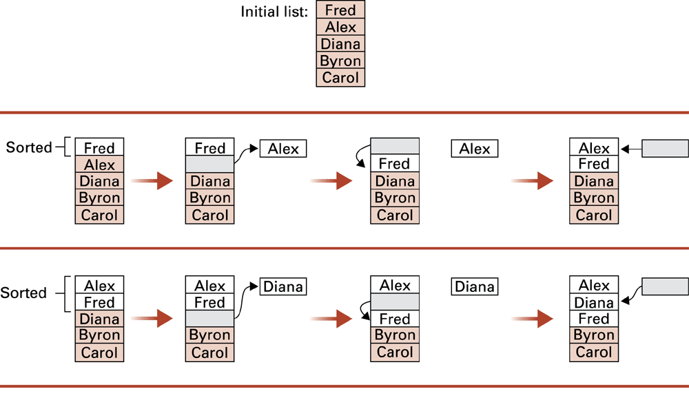
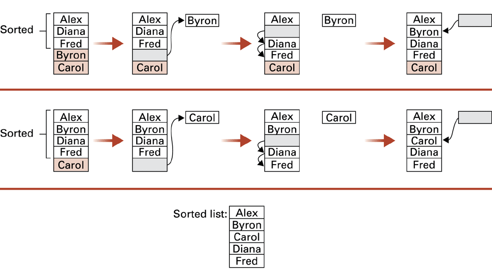
Insertion sort begins with a one-element sorted prefix. Save the next entry as the key, move larger prefix entries one position to the right, then put the saved key into the gap. Saving the key matters: shifting should not overwrite the value that will be inserted. Repeat until the prefix includes the whole array.
Check: Why is checking only a[0] ≤ a[1] ≤ … insufficient as a sorting test?
The algorithm might have lost, duplicated or changed entries. Also compare the output’s values and multiplicities with the input.
10. Trace insertion sort, including equal keys
| Stage | Whole array | Sorted prefix |
|---|---|---|
| Initial | 7, 3, 5, 3 | 7 |
| Insert 3 | 3, 7, 5, 3 | 3, 7 |
| Insert 5 | 3, 5, 7, 3 | 3, 5, 7 |
| Insert final 3 | 3, 3, 5, 7 | All four |
For the final insertion, save the last 3. Shift 7 and 5 right; stop at the earlier 3 because it is not greater than the key. Insert the saved value just after that earlier equal value. Shifting only entries greater than the key preserves the relative order of equal keys, making this version stable. Stability matters when equal-key entries have other information, such as their original arrival order.
The invariant is that the prefix before the next key is sorted and contains the corresponding processed entries. Inserting the key preserves both ordering and those entries. The unprocessed portion gets shorter. This explains the method beyond a single successful trace.
Check: If the two 3s are labelled 3A and 3B in their original arrival order, what should a stable result preserve?
3A should still precede 3B. Their keys are equal, so numerical order alone would not reveal a reversal.
11. The input order changes insertion-sort work
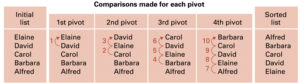
For reverse-sorted distinct values, the usual insertion sort performs 1 + 2 + … + (n − 1) key comparisons and shifts. This sum is n(n − 1)/2: 4,950 at n = 100 and 499,500 at n = 1,000. We are counting comparisons between the key and an array value, not every loop-bound comparison or machine instruction.
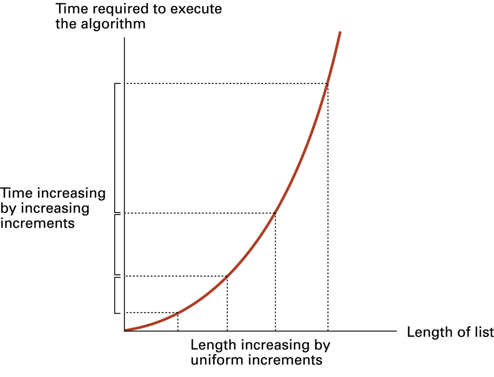
Already sorted input behaves differently: each key is compared with its immediate predecessor, no entries shift, and there are n − 1 key comparisons for n ≥ 1. Thus the standard method has linear best-case and quadratic worst-case growth. Empty and one-element arrays require no insertion passes. Saying merely “insertion sort is quadratic” hides the case being discussed.
Check: Must doubling n exactly quadruple n(n − 1)/2?
No. The ratio approaches four as n grows, but the lower-order term affects small cases. The growth class describes scaling rather than an exact equality for every n.
12. Read the bounds rather than counting loop keywords
Two consecutive traversals of n elements perform n + n = 2n visits, which is linear. A loop over r rows with a complete c-column traversal inside it performs rc visits. If both dimensions equal n, that becomes n². If c is a fixed constant such as four while r grows, the work is linear in r.
Nested loops can also form a triangle: 1 + 2 + … + (n − 1) visits, as in insertion sort’s worst case. Conversely, a loop that repeatedly halves an interval has logarithmic iterations. Its update rule, bounds and per-iteration work determine cost; the visual appearance of the code does not.
When input size means the total number N of cells in an r-by-c table, visiting every cell once is Θ(N). When n denotes a square table’s side length, the same traversal is Θ(n²). These statements agree because N = n². Always define the variable used to express size.
Check: A three-row table gains more columns, and each cell is visited once. Is “two nested loops means quadratic” a correct explanation?
No. With three fixed rows and c columns, there are 3c visits, linear in c and in the total number of cells. Quadratic in n applies when both dimensions grow as n.
13. Representation can change a problem-solving strategy
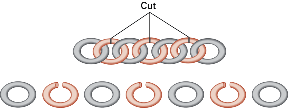
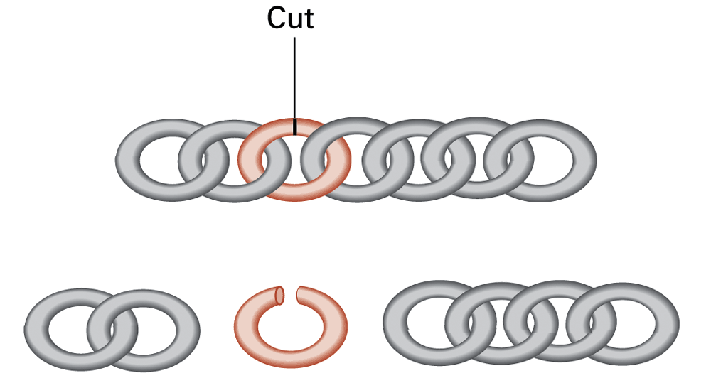
A hotel charges one gold-chain link per night for seven nights. You must settle the correct total each night, and the hotel may return earlier pieces as change. The task is to minimize the number of links cut. Here “one cut” means opening one selected link so it can be removed; the link keeps its value and can be paid as a piece.
| Night | Pieces | Total |
|---|---|---|
| 1 | 1 | 1 |
| 2 | 2 | 2 |
| 3 | 2 + 1 | 3 |
| 4 | 4 | 4 |
| 5 | 4 + 1 | 5 |
| 6 | 4 + 2 | 6 |
| 7 | 4 + 2 + 1 | 7 |
On night two, give the two-link piece and receive the single link back. On night four, give the four-link piece and receive the one- and two-link pieces back. The values 1, 2 and 4 behave like binary place values. The useful representation is the set of payable totals, rather than an instruction to separate every link. Zero cuts cannot settle the first night using an intact seven-link chain, so the one-link-cut solution is optimal under these rules.
Check: Does the solution still apply if the hotel refuses to return change?
No. Exchanges are essential. The method solves the stated problem with change allowed; removing that assumption changes the problem.
14. A batch of readings and a bounded sum
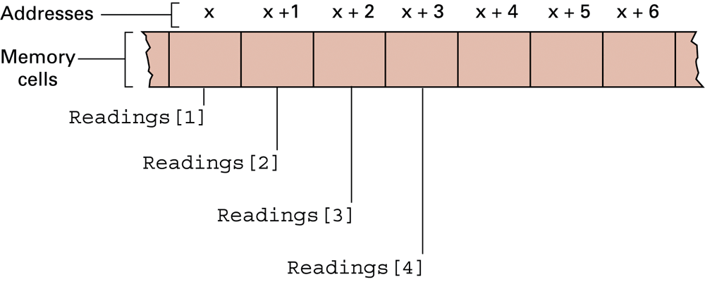
Consider four illustrative ADC counts: 120, 400, 650 and 230. Their sum is 1,400 and their mean is 350. The values are treated as counts on a stated 0–1023 scale, not as universal specifications for every Arduino board or as temperatures. Units and the meaning of a value remain part of the data contract.
#include <stdio.h>

int sum(const int a[], int n) {
    int total = 0;
    for (int i = 0; i < n; ++i) {
        total += a[i];
    }
    return total;
}

int main(void) {
    int readings[4] = {120, 400, 650, 230};
    int total = sum(readings, 4);
    printf("sum: %d\n", total);
    printf("mean: %.1f\n", total / 4.0);
    return 0;
}
For this helper, require 0 ≤ n ≤ 12, at least n accessible elements, and values in 0–1023. The largest permitted total is 12 × 1023 = 12,276, within the guaranteed positive range even for a 16-bit int. This is a deliberate bound; the same function is not an unlimited sum of arbitrary integers.
| Index visited | Added value | Total afterward |
|---|---|---|
| 0 | 120 | 120 |
| 1 | 400 | 520 |
| 2 | 650 | 1170 |
| 3 | 230 | 1400 |
After i visits, total equals the sum of elements before index i. At i = 4 the loop stops without accessing a[4]. For n = 0, the sum is zero; a mean needs a separate decision because division by zero is invalid. The complete example has four elements, so its division is defined. Using 4.0 requests floating-point division rather than discarding a fractional part.
Check: If the count is allowed to grow without limit, can we keep claiming that int is large enough because every sample is at most 1023?
No. The total depends on both the sample range and the number of samples. Revisit the bound, representation or overflow-handling policy when the contract changes.
15. Rows, columns and storage offsets
| Batch / position | 0 | 1 | 2 | 3 |
|---|---|---|---|---|
| 0 | 120 | 400 | 650 | 230 |
| 1 | 300 | 310 | 290 | 300 |
| 2 | 800 | 100 | 900 | 200 |
Rows identify batches; columns identify successive positions within each batch. readings[2][1] refers to the third batch’s second sample, 100. The table’s dimensions belong to the input interpretation. No matrix algebra is required to visit these values.
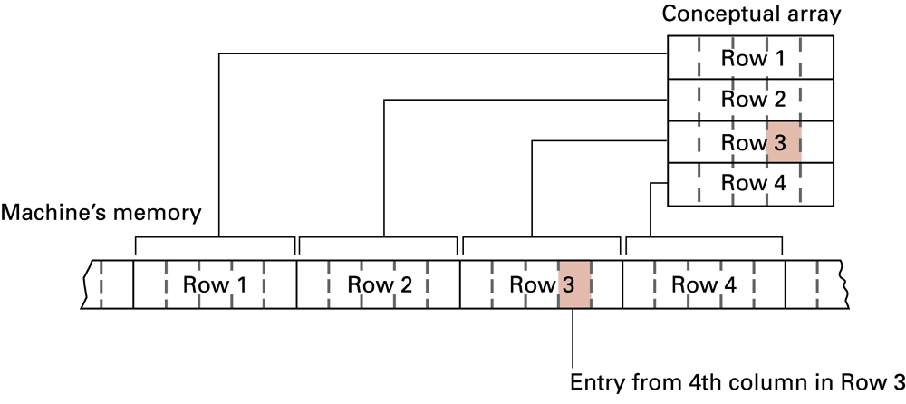
A true C two-dimensional array is an array of row arrays. In int readings[3][4], each row has four consecutive integers, and rows are consecutive. For valid indices r and c, the element is r × 4 + c elements from the beginning; [2][1] is nine elements from the beginning. Its byte offset is 9 × sizeof(int). An int is not universally four bytes.
This storage relationship does not legalize an invalid subscript. readings[0][4] is outside the first row, even though another row follows in storage. Use the appropriate bound for each dimension. Similarly, readings[3][0] exceeds the row count. The GNU C discussion of multidimensional arrays explains arrays of arrays and consecutive row storage.
Check: What is the element offset of readings[2][3] in the 3-by-4 example?
2 × 4 + 3 = 11 elements, or 11 × sizeof(int) bytes. It is the twelfth element, with a zero-based offset of eleven.
16. Nested loops and accumulator placement
#include <stdio.h>

int main(void) {
    int readings[3][4] = {
        {120, 400, 650, 230},
        {300, 310, 290, 300},
        {800, 100, 900, 200}
    };
    for (int r = 0; r < 3; ++r) {
        int total = 0;
        for (int c = 0; c < 4; ++c) {
            total += readings[r][c];
        }
        printf("%d %.1f\n", total, total / 4.0);
    }
    return 0;
}
For row 0, the inner loop visits columns 0, 1, 2 and 3. When the outer loop advances to row 1, the inner loop initializes c to zero again. There are 3 × 4 = 12 body executions. Resetting total inside the outer loop gives one fresh accumulator per row.
| Batch | Sum | Mean |
|---|---|---|
| 0 | 1400 | 350.0 |
| 1 | 1200 | 300.0 |
| 2 | 2000 | 500.0 |
Moving total’s initialization before both loops changes the meaning to an accumulated total across rows. At the end it is 4,600; printing after each row would show 1,400, 2,600 and 4,600. Resetting total inside the inner loop instead loses the earlier values in that row. Initialization placement is a statement about which history should be retained.
Check: If a row contains all zeroes, should the previous row’s nonzero total affect its result?
No. A row total starts at zero for that row. An unexpected carried value indicates that the accumulator was not reset at the intended boundary.
17. A column answers a different question
| Column | Values | Total |
|---|---|---|
| 0 | 120, 300, 800 | 1220 |
| 1 | 400, 310, 100 | 810 |
| 2 | 650, 290, 900 | 1840 |
| 3 | 230, 300, 200 | 730 |
To compute one total per column, hold the column fixed while visiting each row, then reset for the next column. The four column totals also add to 4,600. Agreement between the sums of row totals and column totals is a useful consistency check, although it does not by itself prove that each individual total is correct.
Columns are meaningful only if sample positions align across batches. A missing reading should not silently shift the remaining values into different positions. Sorting each row would also destroy the correspondence between a column and its original time position. Preserve capture order, or clearly state that a transformed copy answers a different question.
For Lab 7, start with saved data so expected results are reproducible. The planned progression protects a one-dimensional traversal before a small two-dimensional adaptation. Capture and transport helpers can supply data; this reading adds no required sorting benchmark, three-dimensional implementation or new hardware.
Check: Can two wrong row totals still add to the correct grand total?
Yes. One can be too large by the same amount that another is too small. Check individual expected totals as well as aggregate consistency.
18. Optional C reference: complete search examples
The program below implements the earlier contracts. The linear search returns the first match. The binary search accepts any matching index and requires ascending input. Both receive a nonnegative int n with at least n accessible elements; neither changes the array. The inclusive interval starts at 0…n−1, which is empty when n is zero.
#include <stdio.h>

int find(const int a[], int n, int target) {
    for (int i = 0; i < n; ++i) {
        if (a[i] == target) return i;
    }
    return -1;
}

int binary(const int a[], int n, int target) {
    int lo = 0, hi = n - 1;
    while (lo <= hi) {
        int mid = lo + (hi - lo) / 2;
        if (a[mid] == target) return mid;
        if (a[mid] < target) lo = mid + 1;
        else hi = mid - 1;
    }
    return -1;
}

int main(void) {
    int unsorted[4] = {18, 7, 31, 12};
    int sorted[7] = {3, 7, 12, 18, 24, 31, 45};
    printf("linear: %d\n", find(unsorted, 4, 31));
    printf("binary: %d\n", binary(sorted, 7, 31));
    printf("missing: %d\n", binary(sorted, 7, 30));
    printf("empty: %d\n", binary(sorted, 0, 31));
    return 0;
}
Expected outputs are linear: 2, binary: 5, missing: −1 and empty: −1. Test first and last elements, missing values below and above the range, missing values between entries, one-item input and duplicates. For binary search with duplicates, check that a returned index is valid and contains the target; do not insist on the first occurrence unless the contract and implementation are changed.
Check: For sorted data 3, 3, 3, can this binary search legally return index 1?
Yes. The midpoint already matches, and the contract permits any match. A first-occurrence search needs additional logic and a stronger postcondition.
19. Optional puzzle: use an ambiguous sum as evidence
Three children have positive integer ages whose product is 36. Their sum equals a house number known to the questioner. Even after seeing the number, the questioner needs another clue. The final clue says there is a unique oldest child. The important information is not just the sum: it is that the sum did not yet determine the answer.
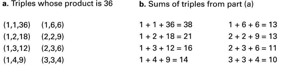
Listing triples in nondecreasing order avoids counting rearrangements as different possibilities. Only sum 13 is ambiguous: 1, 6, 6 and 2, 2, 9. The first has two children tied for oldest; the second has a unique oldest child, so the ages are 2, 2 and 9. The reasoning depends on the stated integer-age model and the unique-oldest wording.
Check: Why would the product 36 and “an oldest child” alone not determine the ages?
Several factor triples have a unique largest entry. The additional evidence that the known sum was ambiguous narrows the possibilities to the two sum-13 triples.
20. Optional reference: recursive search and stored data
A recursive procedure solves a smaller instance by calling itself. A base case finishes without another call. Binary search can be described recursively or with the iterative interval used above. Halving the candidate set explains the logarithmic probe count in either form; recursion itself does not create that advantage.
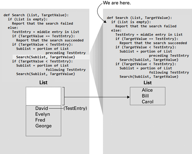
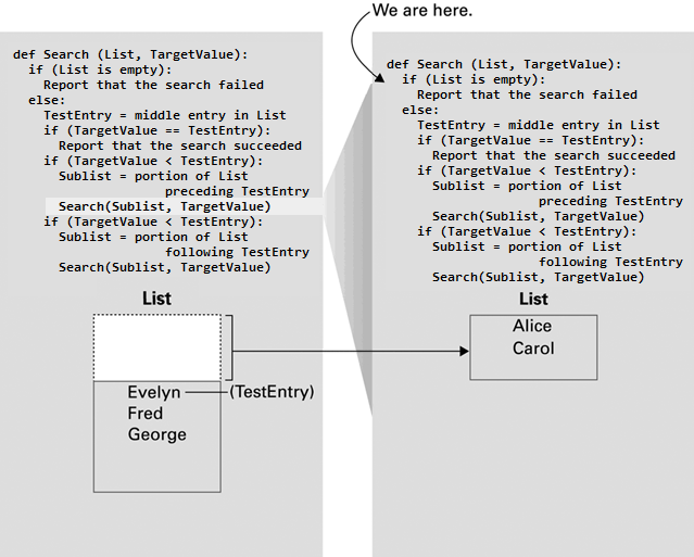
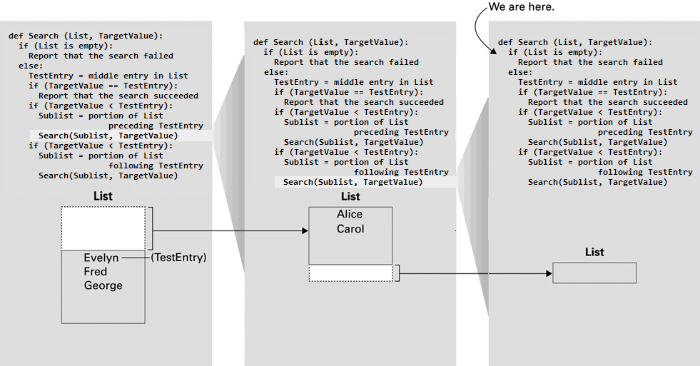
The caller waits while the smaller search runs; the base case stops the chain of calls. In the original images the final comparison mistakenly repeats the less-than test. A larger target must select the following sublist. Read the images for nested-call structure, not as code to copy unchanged. In a real implementation, passing bounds avoids the cost of physically copying each remaining sublist.
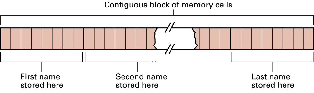
A fixed-size slot layout permits calculating where a selected entry begins. Variable-length strings require additional representation decisions, introduced later. The representation determines whether choosing a middle entry is a direct indexed operation or requires extra traversal. Algorithm analysis must include those underlying access costs.
Check: Does replacing an iterative algorithm with a recursive one automatically improve its growth class?
No. Examine how much smaller each subproblem becomes and what work occurs at each call. Recursion is a way to express control, not a guarantee of efficiency.
21. Further study and review
Explain why ordering permits elimination, trace both successful and unsuccessful searches, preserve values during sorting, and distinguish best, worst and assumed average cases. When comparing cost, name the operation, input-size variable, preparation and memory assumptions. For arrays, predict index ranges and explain where each accumulator is reset.
- Brookshear and Brylow, Computer Science: An Overview, 12th Global Edition (2015), Chapter 5: algorithm representation, problem solving, iteration, recursion, efficiency and correctness. Chapter 8 provides further context for data representations. Original instructor Sets 7 and 8 supply the retained visual examples; legacy figure numbering does not establish an edition by itself.
- Frank Pfenning, CMU 15-122: Binary Search (30 January 2014). A deeper account of contracts and invariants. Compare its interval convention carefully with the inclusive bounds in this reading.
- GNU C: Multidimensional Arrays. Read arrays of arrays and storage order alongside the batch examples.
- GNU C Language Introduction and Reference Manual. Consult array access, integer arithmetic and loops; distinguish standard C from explicitly marked GNU extensions.
All 19 teaching figures from the current Week 8 slides are retained, including insertion-sort enlargements, the ordered tree, original puzzles and optional recursive-search images. Click an image to enlarge it. Historical labels and known source errors are explained alongside the figure. These examples support reasoning; implementing every reference algorithm is not an added lab requirement.